New rate decline EUR model for unconventional reservoirs

Historically, engineers have used Arps’ empirical rate decline model to estimate ultimate recovery in all types of reservoirs.¹ However, its misapplication to wells in unconventional reservoirs often yields overly optimistic results, due to illogical assumptions about boundary-dominated flow, constant bottomhole pressure and isotherm (adsorbed) gas.

These issues led various authors to propose different rate decline correlations, to more accurately model the rate-time behavior of unconventional reservoirs.^2–6 Although these new correlations do an acceptable job of modeling the rate-time behavior of unconventional reservoirs, they are relatively complex and can be difficult to implement. To accurately forecast production and estimated ultimate recovery (EUR) from wells in unconventional reservoirs, a new algorithm is required. 

BACKGROUND

When preforming decline curve analysis (DCA) for unconventional reservoirs (shale reservoirs, tight gas, coalbed methane), engineers must understand that no simplified rate decline model can accurately capture all elements of a well’s short-, medium- and long-term flow characteristics. In addition, no rate decline model can be expected to provide a completely unique forecast of future performance or EUR. We must be practical when attempting to characterize production performance from systems, where the permeability is on the order of nano to micro Darcy (nd/µd 1x10^–6 to 1x10^–3 md). Additionally, the reservoir flow system is complex, and although a naturally occurring or man-made fracture system enables the well to produce, we have only the most rudimentary understanding of the flow structure in either type of fracture system.

Production data from unconventional reservoirs exhibit extensive periods of transient (linear and bilinear) flow behavior, due to low/ultra-low permeability. This often leads to an over-estimate of gas-in-place/reserves when using the conventional rate-time relations (exponential and hyperbolic rate-time relations). A common practice for reserves estimation in unconventional reservoirs is to use the hyperbolic relation and constrain the ultimate extrapolation by including a terminal exponential decline value, or, a “modified hyperbolic” designation. The hyperbolic rate decline relation is expressed as:

              (Eq.1)

In an attempt to better represent the general character of production data for a multi-stage, fractured horizontal well in an ultra-low permeability reservoir, numerous authors have developed rate-time models using specific assumptions to best represent a particular scenario. These rate-time models include:

•   Power-law exponential model 
•   Stretched exponential model 
•   Logistic growth model 
•   Duong model

Each model has strengths and weaknesses. For example: the stretched exponential model is essentially an infinite sum of exponentials; the power-law exponential model is essentially the same as the stretched exponential model (except for a constraining variable). Equations 2–4 present the basic definitions used in all rate-time decline models.

              (Eq. 2)

(Definition of the decline parameter) 

              (Eq. 3)

(Definition of the loss-ratio)

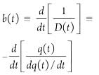              (Eq. 4)

(Derivative of the loss-ratio, b(t))

The rate decline equations for the most common models used today are presented as Equations 5–8:

              (Eq.5)

[Power-law exponential model (PLE)]

              (Eq. 6)

[Stretched exponential model (SEPD)]

              (Eq. 7)

[Duong model (Doung)]

             (Eq. 8)

[Logistical growth model (LGM)]

The source papers should be consulted for definitions of terms and derivations for the applicable model. These four rate decline models, plus Arps, can be used to make long-term rate forecasts, as well as predictions for estimated ultimate recovery. However, all models have varying degrees of difficulty when generating the constants used within each equation.

POWER LAW MODEL

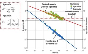
Based on extensive observations of a log-log based linear trend of the D(t) parameter (Fig. 1), engineers determined that it can be modeled with a power-law function (straight line function on a log-log plot). Based on this observation, a simple empirical rate-time decline model q(t) = q_it^–α was developed⁷ by assuming that D(t) = αt^–1. However, this empirical model had the same limitations as the Arps equation, in that a terminal decline rate had to be imposed on the model to properly forecast the well’s long-term behavior.

Fig. 1. Results of computed D and b parameters.^2,3

 
Subsequently, the LeBlanc-Okouma Power Law (LOPL) was developed as an extension of the original empirical correlation through the addition of a late-time term in the D(t) power-law equation (Eq. 9). The ξt term is a factor that becomes dominant at late-time, with the Xi (ξ) term defined as a constant, derived from production history.

              (Eq. 9)

The derivation of the LOPL decline model is presented in Fig. 2.

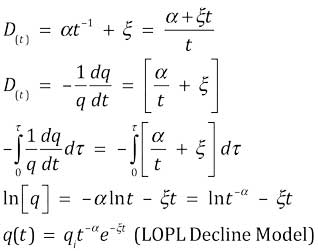
Fig. 2. Derivation of  LeBlanc-Okouma power law model.

              (Eq. 10)

In equations 9 and 10, qi is the initial rate for the model; t is time in days; and α and ξ are constants obtained through history matching of the well production data. The LOPL equation can model the transient and transition flow regimes through the power law term and the boundary-dominated flow regime through the exponential term.

LOPL MODEL (UNCONVENTIONALS)

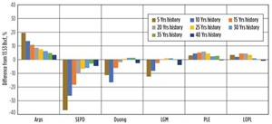
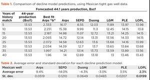
Although numerous wells have been used to validate the LOPL model, a single example is highlighted to compare the forecastability of all rate decline equations. The case history producer is a Mexican tight-gas well with 44.1 years of production data. The authentication process restricted the history match period to a subset of the production data and then generate forecast production as follows; 1) match all models; 2) forecast each model to the end of the actual history; and 3) compare the results of each model to the actual production. Figure 3 and Table 1 present the comparative results for the indicated decline models. Table 2 presents the average error and standard deviation for each model. 

Fig. 3. Percent difference in recovery forecast, based on history-matched time period.

 
From these results, the LeBlanc-Okouma Power Law model yielded a consistently lower error, and a lower overall standard deviation in the forecasted 44.1-year production for all history match periods. The Arps model consistently over-predicted the 44.1-year production, and the SEPD model consistently under-predicted the production. Overall, the LeBlanc-Okouma Power Law and the Power Law Exponential yielded the most consistent errors and lowest standard deviation.

LOPL MODEL (CONVENTIONAL) 

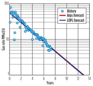
The LOPL model is also valid for conventional reservoirs, as demonstrated by the comparison of a North Sea well, Fig. 4. The plot shows the history match and forecast for Boyle field in Quadrant 49 of the North Sea. Both the Arps and LOPL forecasts are equivalent.

Fig. 4. LOPL decline forecast versus Arps in conventional reservoir, Boyle field, North Sea.

  
The Arps profile was generated using b=0 (exponential decline) and a daily decline factor of 0.0008482. The LOPL profile was generated using α of 0.0001003 and ξ of 0.0008491. Both models had q_i of 53.6 MMscfd. After 13 years of production, Arps predicted EUR of 63.6 Bscf. The LOPL model was 63.5 Bscf. 

MODEL BENEFITS 

The LeBlanc-Okouma power law decline model offers users a real-world algorithm to forecast EURs in unconventional reservoirs, including shale gas, liquids rich shale, tight gas sands and coalbed methane. The LOPL decline model is easily applied. It includes a late-time exponential term ξt in the equation, to enable accurate modeling of transient, transition, and boundary-dominated flow. 

The LOPL model yields more consistent estimates of short-to-long-term production in unconventional reservoirs, compared to other time-rate models, while retaining the capability of modeling conventional reservoirs. 

REFERENCES

1.   Arps, J. J., “Analysis of decline curves,” Trans. AIME 160: 228–247, 1945.
2.   Ilk, D., A. D. Perego, J. A. Rushing and T. A. Blasingame, “Exponential vs. hyperbolic decline in tight gas sands, understanding the origin and implications for reserve estimates using Arps' decline curves,” SPE paper 116731, presented at the SPE Annual Technical Conference and Exhibition, Denver, Colo., Sept. 21–24, 2008.
3.   Ilk, D., J. A., Rushing and T. A. Blasingame, “Decline curve analysis for HP/HT gas wells: Theory and applications,” SPE paper 125031, presented at the SPE Annual Technical Conference and Exhibition, New Orleans, La., Oct., 4–7, 2009.
4.   Valkó, P. P., “Assigning value to stimulation in the Barnett shale: A simultaneous analysis of 7000 plus production histories and well completion records,” SPE paper 119369, presented at the SPE Hydraulic Fracturing Technology Conference, College Station, Texas, Jan. 19–21, 2009.
5.   Clark, A.J., L. W. Lake and T. W. Patzek, “Production forecasting with logistic growth models,” SPE paper 144790 presented at the SPE Annual Technical Conference and Exhibition, Denver, Colo., Oct. 30–Nov. 2, 2011.
6.   Duong, A. N., “Rate-decline analysis for fracture-dominated shale reservoirs,” SPE Reservoir Evaluation and Engineering 14 (3), pp 377–387, 2011.
7.   LeBlanc, D., “Petroleum engineering essentials: Tools and techniques to evaluate unconventional (and conventional) wells and reservoirs,” 198–199, self-published book available online at http://www.eastexpetroleum.com/PE_Essentials/Book.html.