Lifecycle performance of WET (subsea) and DRY Tree systems for big, complex reservoirs in ultra-deep waters

To remind readers, Frontier Deepwater’s three World Oil articles in 2020 and 2021 covered the savings and value created by adopting a phased dry tree development concept, rather than a risky and expensive hub-spoke subsea (wet tree) development scheme, extrapolated from industry’s Miocene experience. Frontier presented research that used public domain information from the BSEE Gulf of Mexico database to clarify how, and why, the industry’s efforts to exploit massive discoveries in the once promising but deeply challenging Lower Tertiary Wilcox trend have failed commercially. While project organizations within the major players seem content with their hub-subsea development schemes, drilling and reservoir groups are well-aware of these failures and the documented problems. 

The first part of this year’s three-part series (published in World Oil last month) presented the method, modeling assumptions, and high-level results of simulated operations for a ten-well ultra-deepwater field development. The simulations, covering a wide range of sensitivity cases, were generated by BMT’s SLOOP event domain software, using realistic system and metocean models to cover a 30-year project life. The results led to important conclusions about the differences in operating lifecycles: 

The Dry Tree option is expected to provide at least $20 billion of higher value. 

• The “DRY Tree” field phased approach (using two “FrPS” platforms) is expected to recover ~31% more of the reserves in the first 20 years of production from the modeled reservoir, yielding over $10 billion more in revenue (at $100/bbl) during that period, as compared to the analogous WET tree subsea/hub scheme; this is $6.3 billion more revenue in the first 10 years. 

• While Frontier’s FrPS DRY tree development is generating at least $10 billion more revenue, the WET/subsea tree scheme is spending almost $10 billion more on operations. 

UNDERSTANDING RESULTS FROM SIMULATING LIFECYCLE OPERATIONS 

First, for convenient reference, we return to the comparison of the production profiles for the competing field development options, Fig. 1. The SLOOP software and case models were described in Part 1. The chart shows the mean, as well as the P10 and P90 percentiles of the average annual production rate. For the FrPS (Dry Tree) case, there are four distinct peaks in production rate, corresponding to completing all wells at each well center and, later, sidetrack/recompletion of the wells. 

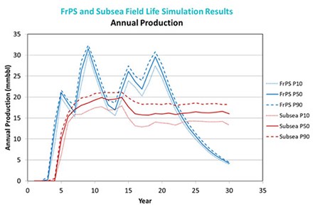
FIG. 1. Comparison of simulated production profiles. 

For the subsea (Wet Tree) case, there are no such distinct peaks; the peak production is much lower and occurs much later in the field life. Also, there is more spread between the P10 and P90 production ranges. These shortcomings are seen in part, because the many efforts to run and retrieve the drilling riser and subsea BOP are significantly affected over time by metocean conditions (especially loop currents and hurricanes). 

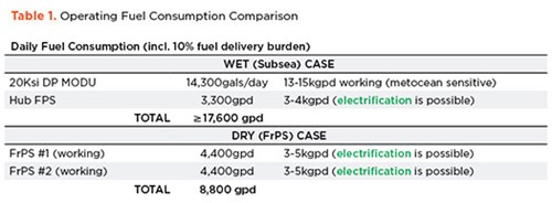
While not directly incorporated into the dynamic simulation of the project, fuel consumption is an important part of operating costs and pollution. The information in Table 1 is used to estimate these costs for economic and environmental considerations. 

Understanding the simulation results. The following discussion and charts are intended to help the reader more deeply understand the main conclusion of Part 1. Figure 3 in Part 1 showed the 20-Ksi DP MODU staying busy, once it arrives at the field; however, there was no period of time where both of the FrPS rigs would be fully utilized. 

Except for the rig utilization chart discussed above, the results from simulations presented in the preceding article may appear somewhat simplified and smoothed, belying the detail of analysis behind what was reported. For example, it is worth considering how the statistics plotted in the following chart (Fig. 2) are assessed through compilation of 240 runs of the simulated 30 years of project duration. The time history of production from one “realization” (time history) for the WET case is overlaid on the statistical curves produced by data from all 240 realizations. This indicates how the monthly average production rate from “one life history” can exhibit substantial variability. 

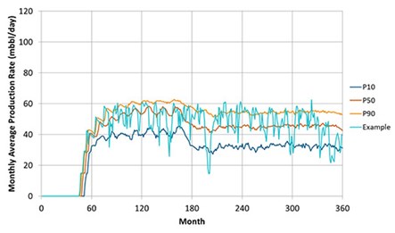
FIG. 2. Monthly average production rate for one realization, plotted over the statistics for all realizations. 

The P50 curve for the 20-Ksi DP MODU utilization curve, shown in the preceding article, might cause the operator’s asset manager to expect that the MODU will be too busy to ever be allowed to leave the field. However, if the operator adopts a policy allowing the 20-Ksi DP MODU to leave the field, then situations can occur where production in this field drops, because a backlog of service requests builds for several wells before the 20-Ksi MODU returns. The model adopted for this study does allow the 20-Ksi DP MODU to leave the field, if no backlog of requests exists when it finishes a service request. Then, the MODU has “free time” to work away from the field until new service requests start popping up. Unfortunately, the MODU cannot return immediately. So, a backlog of service requests begins to accumulate. 

The big drops in production rate seen in the “Example” curve of Fig. 2 could be due to an extended absence of the MODU or, possibly, to hurricanes. The following charts provide insights into how various causes of downtime play into the overall history of well service delays and interruptions of production. All in all, even though it is expensive to have the rig stay in the field when idled, the operator’s asset manager would be tested severely in making a decision that would allow the highly specialized and expensive 20-Ksi DP MODU to leave the field. 

Figure 3 shows how much time the 20-Ksi DP MODU is predicted to be away, if the operator’s policy allows temporary demobilizations. For about 11% of the realizations, it never gets away from the field. If it does demobilize, there is a 50% likelihood that a service request will pop up within ~32 days. The “time to return” adds the assumed “rig remobilization response time” distribution to the statistics for time until a first service request (the light blue curve in Fig. 3). So, the result is that there is a 50% likelihood that the rig will make it back to the field within ~224 days. This means that if the MODU does demobilize from the field, there is a good chance that several service requests will have piled up before the MODU makes it back into service at the field, and production may be dropping off. 

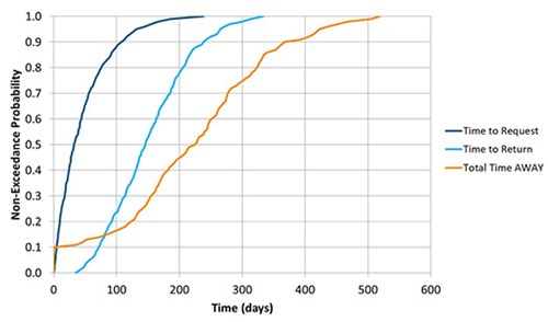
FIG. 3. 20-Ksi DP MODU remobilization statistics. 

Figures 4 and 5 show us how the service request (workload) backlog builds while the MODU is away. Figure 4 indicates that while there is ~17% chance that only one service request will be waiting, there is just over a 60% likelihood of three or more service requests and an almost 30% chance that more than four jobs will be waiting when the MODU returns to the field. Figure 5 reveals a few instances where more than six jobs ended up being backlogged. 

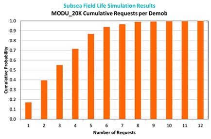
FIG. 4. Cumulative probability of the 20-Ksi MODU’s work backlog. 

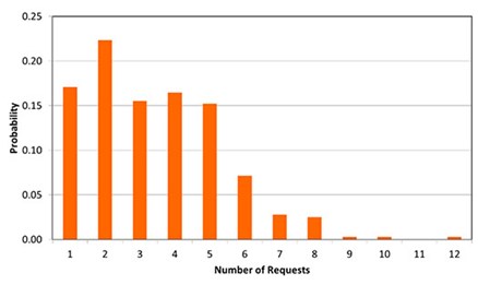
FIG. 5. 20-Ksi DP MODU service request backlog statistics.  

When asset managers have this kind of information at their fingertips, they will fight hard to keep the 20-Ksi DP MODU permanently located at the field—even if it could be “idle” for a month or two! While the WET Case model for this study does allow the 20-Ksi DP MODU to leave the field to work elsewhere, the model does not consider absences for periodic drydocking/maintenance. Such an absence would be extended for several months. 

Thus, while preventing the MODU from leaving the field during idle times would tend to increase the cumulative lifetime production for the WET case by some amount, sending the MODU away for drydocking every five-or-so years would seriously decrease the cumulative production. These offsetting factors mean that the current WET case model presents a reasonably realistic picture of production/reserves recovery over the simulated time history of the project. 

UNDERSTANDING “WELL DOWNTIME” AND “RIG NON-PRODUCTIVE TIME” 

We now have a picture of how demobilizations affect the working performance of the 20-Ksi DP MODU, but what happens when it and the FrPS units are actively attempting to perform their intended operations at the field? Both the DRY tree platforms (the FrPS units) and the 20-Ksi DP MODU will experience metocean conditions and equipment failures that halt or delay operations. The following charts explore these influences and the differences between the WET case subsea well systems and DRY tree systems with direct surface access to the wells. 

The time needed to complete any well operation accounts for interruptions due to unfavorable metocean conditions (including hurricanes as well as high winds, waves and currents) and BOP failures (as the only type of equipment failure modeled). Even though predicted and actual arrival of hurricanes completely shuts down well operations for both cases, a DP MODU—and its interface with the well it is servicing in ultra-deep water—is much more sensitive to troublesome metocean conditions than the permanently moored FrPS units with permanently attached, fully redundant tie-back risers. In addition, when a hurricane threat is past, it takes longer for the DP MODU to restart well operations. The following charts show how the modeled sensitivities have resulted in substantial differences in performance for the competing systems. 

It is no surprise that there are many events that cause interruption of well servicing operations for both DRY and WET systems. Figure 6 confirms this expectation. In the early years, when the DRY scenario has a 15-Ksi DP MODU deployed to the field to perform pre-drilling at the two well centers, it is subject to a high degree of interruptions. Once a DP MODU is no longer needed, the number of interruptions drops dramatically—even though two FrPS units are working in the field. There are a couple of jumps in the number of interruptions when sensitive operations occur during the periods when the FrPS units are performing sidetracking and recompletions (years 13-14, 17-18). 

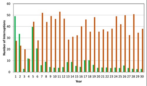
FIG. 6. Mean number of interruptions each year: All causes. 

As a result, one would expect that throughout the producing life of the field, the 20-Ksi DP MODU servicing the wells of the WET case will experience a lot more Non-Productive (rig) Time (the much hated NPT). Figure 7 confirms this expectation, which impacts the “Well Downtime.” 

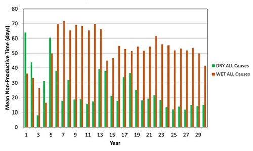
FIG. 7. Mean total annual rig Non-Productive Time: All causes. 

During the early years,the 15-Ksi DP MODU, working for the WET case, spends less time in the field, because it has less to accomplish. As a result, the WET case experiences less NPT in years 1-6. Still, subsea BOP failures feature prominently in NPT (as in the real world). When the 20-Ksi DP MODU arrives, and the 15Ksi MODU moves to Well Center #2, BOP failures dominate NPT for the WET case while both rigs are working. Figure 8 has the WET case’s 15-Ksi MODU finishing up in year 7, but the D&C activities of the 20-Ksi MODU carry a high NPT, due to subsea BOP failures through year 13. Deepsea loop currents and waves are always big part of NPT for the WET case. 

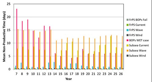
FIG. 8. Mean total annual NPT per cause: Core years.  

It is worth looking more closely at the role that hurricanes play in causing NPT and, indirectly, well downtime and production delays. Figure 9 shows NPT days for both cases during the core years of project life. When the FrPS units of the DRY case are sidetracking and recompleting wells, hurricane-induced NPT rises dramatically. However, for most years, the WET case suffers much more hurricane-induced NPT. On average, the WET case experiences about 50% more hurricane-induced NPT than the DRY case over the core years. The main reason the WET case has so much more NPT, due to hurricanes, is that it takes much longer to retrieve and re-run the riser, reconnect the LMRP, and restart well operations when the 20-Ksi DP MODU returns from a hurricane-induced site abandonment. 

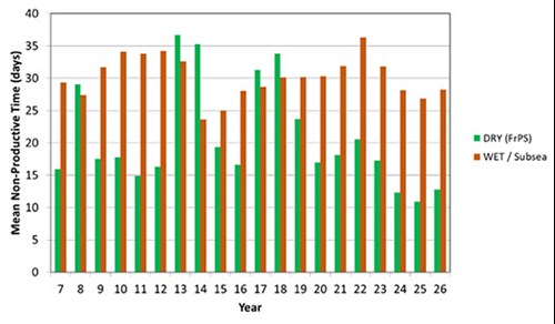
FIG. 9. Hurricane-induced mean total annual NPT: Core years.  

Of course, the DRY case suffers substantial hurricane-induced NPT in the early years, when a 15-Ksi DP MODU is performing pre-drilling operations at the two well centers—even more than the WET case during that time period. The DRY case development plan calls for much more pre-drilling activity by its 15-Ksi MODU and is thus exposed to more hurricane NPT in those early years. This is reflected in Fig. 10. 

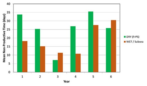
FIG. 10. Hurricane-induced mean total annual NPT: Early years. 

Having looked at all the causes of NPT, it is worth considering how the NPT is distributed across the various types of well operations modeled to see which operations suffer the most NPT. Figure 11 presents the results from the full life simulations (not just core producing years). This chart helps us understand why the DRY case suffers so much NPT during the early years. The NPT of the pre-drilling program for the DRY case is a combination “MODU pre-DRILL to TD” plus “MODU pre-DRILL/Set 14 in” (22.2 days + 10.5 days = 32.7days) that all occurs within the first six years of the project. The NPT of the pre-drilling program for the WET case is just 24.5 days in those years because, in that case, the 15-Ksi DP MODU only drills three wells to Target Depth (TD) at Well Center #1. 

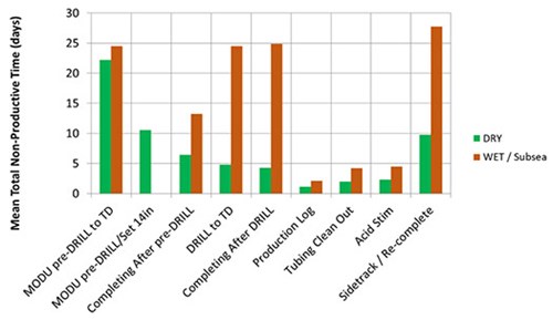
FIG. 11. Mean well operations Non-Productive Time (rig NPT): All causes.  

For the DRY case, just over half of all NPT occurs during the pre-drilling program. For the WET case, only ~24% of all NPT occurs during pre-drilling operations. However, as a key factor in well downtime, the total of the “mean NPT” across all operations is important to keep in mind—with ~126 days totaled across the means for the WET case and only about half as much for the DRY case. 

The two FrPS units will be able to perform more well interventions needed to keep wells producing as intended, which is a key reason for the recovery of an additional 31% of reserves. The following charts confirm that more tubing cleanouts and acid stimulation jobs are performed for the DRY case than for the WET (see Figs. 12 and 13). Every time a stim job or tubing clean out is performed, production from the affected well is interrupted, so it is important that such tasks are accomplished efficiently, as well as safely. Figure 11 did show that there is very little NPT associated with these operations, for either the DRY or the WET case, but it is still clear that the advantage goes to the DRY case. 

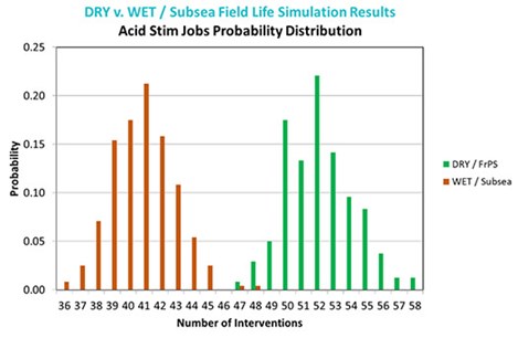
FIG. 12. Probability distributions on the number of acid stimulation jobs (WET v. DRY).

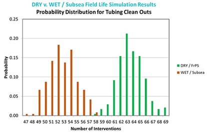
FIG. 13. Probability distributions on the number of tubing clean out jobs (WET v. DRY). 

Remembering that pending interventions have priority over drilling and completing a new well or starting a sidetrack/recompletion, we wrap up this section by considering how all the interventions and delays discussed above impacted full field development. Figure 14 shows the P10 and P90 range for “milestone” well completions and recompletions, with the DRY case completing all ten of its wells within ~8.5 years, while the WET case does not finish until five years later. The sidetracking results are even more disappointing for the WET case, as the tenth sidetrack has ~13% chance of being delayed outside the 30-year window. 

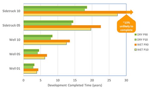
FIG. 14. P10-P90 timing for well completion milestones (WET v. DRY).  

CONCLUSIONS 

Frontier decided to perform what we called a “Green Ops study,” to investigate whether a “Dry Tree” field development was any more efficient and less polluting than the subsea (“Wet Tree”) hub-spoke field development schemes, currently adopted and still favored by operators’ project departments, for deepwater fields in the U.S. Gulf of Mexico. As revealed in Part 1 of this series, we were somewhat surprised that Frontier’s DRY Tree field development plan (using two “FrPS” platforms) would be expected to provide at least a $20 billion increase in value to the asset owners during the core producing years. This second part presents more results of the SLOOP simulations to clarify and support that conclusion while confirming expected reductions in pollution. 

The huge increase in value does not include the front-end savings on field appraisal or CAPEX reduction in field development—or even properly reflect the difference in Expected Net Present Value that comes with full consideration of the time value of money or the big improvement in risk management. It also does not include the increase in Expected Ultimate Recovery from the field that is provided by a dry tree field development. 

When all the differences in value (and the tremendous reduction in emissions and pollution risk) are accounted, it is clearly time for a step-change away from a perspective locked on what have proven to be failed and failing hub-subsea scenarios for the ultra-deep Lower Tertiary Wilcox trend. WO 

Editor’s note: Part 3 of this article series will add analyses of field appraisal and abandonment to further highlight key financial and environmental impacts by reflecting on the concepts of ALARP and AHARP.