Modeling Simian Field's deepwater slope-channel turbidites

Combining deterministic and stochastic methods improves reservoir facies prediction offshore Egypt. 

Mohammed Said, BG Egypt; and Dr. Mohamed Darwish, Cairo University

The giant Simian Field in the West Delta Deep Marine (WDDM) concession offshore Egypt is an area where good 3D seismic coverage, combined with exploration and data acquisition programs, provided the opportunity to investigate a giant Pliocene deep-marine channel complex. After the exploration and appraisal stages, development started quickly. Understanding the reservoir’s internal architecture was a major challenge, since the well logs had considerable heterogeneity. Essential details needed to be reflected in the 3D geological model.

The knowledge gained from the data helped the modeling team create a depositional model of the area. This depositional model, was integrated with pre-stack inverted seismic data and early dynamic data from producing wells, to generate a computerized 3D geological model for the field. The model’s value is derived from integration of the different data types. Early history matching, together with later development wells, verified this work.

Three-dimensional computerized reservoir modeling is becoming one of the most effective tools for reservoir management and development planning. Modeling approaches and software have been developed, which require a deep knowledge of reservoir properties. Simian Field is one of the newly discovered fields that used an integrated reservoir model to help with field management.

NILE DELTA GAS PROVINCE

The Nile Delta occupies the northeastern part of the African continent and is one of the world’s classic deltas. The present-day delta has passed through different events as part of the regional tectonics in the Mediterranean area, which have shaped many of its physiographic features. This area is now regarded as major gas province and one of the most promising areas for future petroleum exploration. In the last decade, offshore exploration using high-quality 3D seismic has resulted in the discovery of significant reserves, 42 Tcf discovered with about 50 Tcf yet to be found.¹ 

The WDDM concession was awarded to BG and Edison in 1995, with Edison’s equity later acquired by Petronas. The license is about 50-100 km offshore in deep water (250-1,500 m). The license covers 8,200 km² of the north-western margin of the Nile Delta cone.

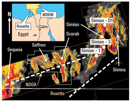
The major tectonic features (controls) in the concession are the SW-NE-trending Rosetta fault and the NNE-SSW NDOA fault, which played significant roles in eustacy control of marine sedimentation throughout the Pliocene and into the Pleistocene. A series of successive successful exploration and appraisal wells drilled by BG Egypt and Rashpetco (a joint venture company) encountered multiple Pliocene gas-bearing sands in slope canyon settings, most of them of Late Pliocene age, Fig. 1.² 

Fig. 1. Simian Field is in the Nile Delta, with Upper Pliocene gas discoveries in the WDDM concession.2

BG acquired four seismic surveys over six years, which helped delineate the gas-bearing sands. The surveys were combined with well data to understand and construct a geological model for the area.

SIMIAN FIELD

Simian Field is in the eastern part of WDDM and was discovered by Simian-1 in 1999. Later, two appraisal wells, Simian-2 and Simian-3, confirmed communication along the main channel. Each of the wells encountered different gas-water contacts, which step down progressively to the north. These were interpreted as perched aquifers. The channel exists at the base of El-Wastani Formation (Late Pliocene), at a similar level to the many slope channels in the offshore Nile Delta area. The field is a stratigraphic/structural trap composed of dip-closure along the northern part, combined with the reservoir pinching out in the southern margins and stratigraphic closure created by lateral pinch-out of the channel along the length of the reservoir. Claystones form the main lateral and top seal to the Simian reservoir. The field is comprised of a number of channels constrained within a NNE-SSW-trending canyon.

Later development wells, Simian-Di and Simian-Dm, confirmed common static pressure communication in the gas leg, and also encountered perched water tables. Simian-2 and Simian-3 were sidetracked and became producers along with the development wells. The field started production progressively from April 2005. In late 2005, two additional development gas wells, Simian-Dp and Simian-Dn, were added. The present production rate is 700 MMcfd.

RESERVOIR MODELING

The modeling work aimed to:

• Characterize the different facies/depositional elements of the Simian channel complex
• Incorporate reservoir sedimentologic and petrophysical information along with seismic data to build a static 3D geological reservoir model as an input for the reservoir simulation process
• Modify the usual static reservoir model workflow to improve and develop a data and integration “best practice.”

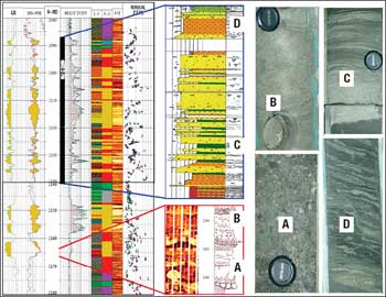
Data types used included lithology, wireline data, formation images and interpretation, petrophysical analysis, and core and production test data from well logs, Fig. 2. Several other data types from seismic were integrated: structural data showing time and depth surfaces and fault polygons, 2D amplitude maps, 3D seismic inversion data and AVO inversion cubes.

Fig. 2. An integration of wireline logs, formation imaging, core description and core photo shows the basal conglomerate (A), massive sand (B), thin-to-medium-bedded facies (C) and thin-bedded facies with soft deformation features (D).2

General workflow. The general workflow was divided into five parts:

A. Definition of the depositional model and identification of the major reservoir elements

B. Analysis of the reservoir facies/elements petrophysically and sedimentologically for the degree of heterogeneity and their relation to the seismic

C. Reservoir modeling (grid design, facies and petrophysical modeling

D. Up-scaling

E. Model validation.

The depositional model for the field is based on previous work done by Cormac and John,3 which included many Pliocene submarine channels drilled in the WDDM concession. The study used the sedimentological interpretation of formation imaging, combined with the 3D seismic data, to build the depositional model and define its developmental stages.

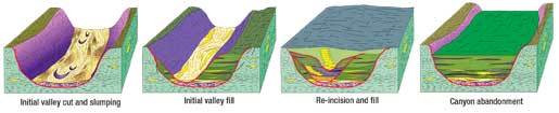
Canyon fill development. The depositional model encompassed four main stages of canyon development and infill: initial valley cut and slumping; initial valley fill; re-incision and fill; and canyon abandonment, Fig. 3.

Fig. 3. An idealized deep marine canyon fill development has several steps.2

Initial valley cut and slumping. The canyon incision phase is defined in two ways. First, there are thin gully-like sands (remnants of erosive gravity flows incising the canyon). Second, there are thick slump units, often with associated debris flows that appear to be collapse of the steeply incised topography.

Initial valley fill. Following canyon incision, the accommodation space was filled by a mixed transgressive fill. Often valley fill begins with the deposition of broad, amalgamated sand sheet across the valley, creating complex channels. Vertical and lateral sand connectivity is likely to be excellent, followed by a variable net/gross succession of thin channel sands, thin flat-bedded sheets, low-density thin-bedded turbidites, slumped shales and hemipelagic shale.

Re-incision and fill. The return of low-stand conditions can cause re-incision of the canyon with a subsequent fill. Re-incision can produce a new succession similar to the initial valley fill, but in general, it produces narrower valleys. Re-incision surfaces are overlain by a stacked succession of thalweg channels. A thalweg is a canyon’s deepest channel path.

Levees. Seismically, levees are identified by their position on either side of the thalweg. In the formation images and core, several criteria can identify channel levees as thin sand and silt laminae. Other criteria can identify creep deformation, which is driven by levee topography. This leads to folding, syn-sedimentary faulting and upward-decreasing depositional dip of thinly laminated sand/silt and shale.

Mixed later incision fill. An interpreter may recognize lower net/gross fill above the incision surfaces. This fill is formed by thin-bedded sands, some thin channels, occasional slumping and hemipelagic shale. Sand deposition is likely to be from distal channel overbank, shallow channels and sheet sand deposition in small lobes.

Canyon abandonment. Termination of coarse-grained canyon fill took place in several ways. The system may have been drowned with minor thin, dilute turbidites of low- to medium-quality thin-bedded facies, until coarse-grained deposition ended. Or, the coarse fill may have been overlain by slumped shales, plugging the system.

SEDIMENTOLOGICAL AND PETROPHYSICAL FACIES ANALYSIS

The model components were investigated and evaluated sedimentologically and petrophysically. Logging suites provided fundamental information for reservoir characterization. Also, each well was calibrated against its corresponding seismic expression to determine the relationship between reservoir facies and seismic data.

Stratigraphic framework. The stratigraphic framework for Simian is simple; the reservoir is found in the Late Pliocene and is composed of a channel complex that runs along a submarine canyon, with some outside runoff. Seismic data revealed and delineated the reservoir framework and extension.

Facies analysis. Sedimentological interpretations based on formation imaging data for Simian wells were done by service companies and were calibrated against core data when available. The number of interpreted litho-facies was reduced to a reasonable number of consistent facies codes that could be handled easily during the modeling, and represent reservoir heterogeneity. Accordingly, the original litho-facies were rationalized into:

• Channel sand: These are good-quality, thick sand bodies, showing erosive features. They represent individual, amalgamated channels or sheet-like sands. This facies deposits sediment, following the principal flow direction down the channel axis. Seismic images reveal the geometry and orientation of gas-bearing sand.
• Minor sand: These are short-lived, individual, good-quality sand bodies from diluted turbidity flows. They are within the reservoir following the main flow direction or may occur within the abandonment phase.
• Thin-bedded levees: This facies is from the relatively sand-rich proximal part of channel levees and is composed of finely laminated (centimeter scale) sand and shale.
• Hemipelagic shale: This is a background facies.
• Debris flow: This muddy, chaotic facies represents the ephemeral phases of gravity flows and/or canyon wall collapse.
• Overbank: This thin-bedded facies is composed of finely laminated (centimeter scale) sand and shale layers from the distal part of channels levees, and the channel abandonment phase.

Petrophysical properties. Effective porosity (_eff) and water saturation (S_w) were obtained from evaluation of conventional CMR and FMI logs. Facies’ petrophysical properties were then computed and statistically analyzed to understand the facies characteristics and reservoir heterogeneity. Data analysis revealed variable porosity across the different facies types and showed the high degree of heterogeneity within the reservoir, Fig. 4.

Fig. 4. Histograms show channel sand (a) and levees (b) for effective porosity (Feff, top) and effective water saturation (Sw, bottom).2

For example, a channel sand had these values: mean = 0.255, minimum = 0.063 and maximum = 0.340 porosity units, while a thin-bed levee had: mean = 0.144, minimum =0.100 and maximum = 0.230 porosity units.

Analysis of S_w revealed variability between the different facies types, which directly affected reservoir quality and hydrocarbon volume. For example a channel sand had: mean = 25.7, minimum = 9.7 and maximum = 56.0% S_w, while a thin-bed levee had: mean = 68, minimum = 57 and maximum = 81.0% S_w.

Correlation showed an inverse relationship between _eff and S_w. Rocks with high _eff possess low S_w and high gas saturation (S_g), and vise versa. This can be attributed to the rock’s shale content. When shale content is low, _eff of clean sand is high and the volume of irreducible water is low, and vice versa. When shale content is high, _eff is reduced and irreducible water volume is high.

Variograms indicate spatial trends and property variation. A variogram model was established for the main facies (channel sand, thin-bed levee and overbank). Other minor facies couldn’t be used due to limited data points. Due to the small number of wells in the 40-km field length, horizontal variograms are of lower confidence relative to the vertical variogram.

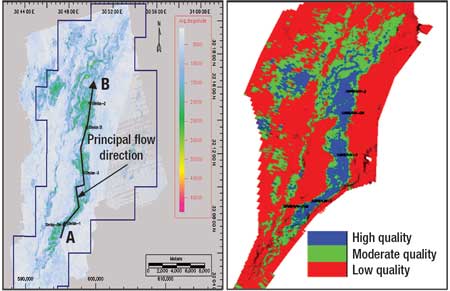
Facies and seismic. Good-quality seismic data provided outstanding help to predict reservoir facies distribution away from well control. Two-dimensional amplitude maps helped quantify facies Net-To-Gross (NTG) percentage relative to the total reservoir volume.

Other maps, such as Average Absolute Amplitude (AAA), resulted from amplitude extractions reflecting the lateral distribution of the gas-bearing facies. AAA enabled modelers to define areas rich in good-quality, gas-bearing facies. Although 2D maps don’t provide information about reservoir facies’ vertical distribution, they are still a valuable tool to define channel core and belt areas, and therefore enable NTG estimation by applying seismic cutoff values to separate high-, mid- and low-quality areas. These cutoffs are based on well penetrations and analog reservoirs. Upon defining the different quality areas, each area’s contribution to the total volume can be estimated and overall NTG calculated, Fig. 5.

Fig. 5. AAA map (left) and quality classes map (right) identified gas sands.

Pre-stack inversion helped to characterize the rock bodies-not their boundary-which guided the modeling software during the facies distribution process. There were two types of inverted seismic data: Poisson’s ratio and facies probability. The seismic data was extracted along the well paths and analyzed for the corresponding facies.

RESERVOIR MODELING

Building the reservoir model was achieved via a series of steps using RMS, a geological modeling software. These steps included: structural model design, population with reservoir facies, population with petrophysical properties, up-scaling and model validation.

The basic grid construction used time and depth surfaces in combination with interpreted faults to build the reservoir’s 3D framework. Faulting in Simian is generally of low importance, compared to stratigraphy. So the time grid was constructed using the time surfaces with no faults for simplification. The grid hosted the seismic data before transferring it to the depth grid, using simple layer-to-layer rescaling.

The structural depth grid used the depth top and base surfaces in combination with faults that were thought to be important. The layers between the top and base were arranged to mimic the natural vertical accretion pattern inside the turbidite channel complexes and to account for erosion and lateral truncations.

The 3D grid is composed of cells, arranged in layers, rows and columns. During modeling, these cells host values representing the reservoir facies and their petrophysical properties. It was crucial to reflect the sediment flow direction and reservoir fluids (flow from aquifer to gas) in the grid design.

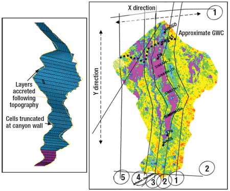
Two grids (geological/fine and simulation/coarse) were designed by manually digitized control lines to ensure that the computer-made grid honored the geology and fluids. Moreover, cells dimensions were controlled to set fine cells at the channel core and coarse cells at distal locations to capture core area details, where most of the wells exist, and, by coarsening up the far cells, reduce the overall number of cells. This has a direct impact on computer modeling time, Fig. 6.

Fig. 6. Structural grid design for the Simian model shows how the layers fill the bottom and are eliminated at canyon walls (left) with the amplitude map (right).

Facies modeling. Facies modeling is the population of reservoir facies within the geological grid. In this step, the geological knowledge about facies arrangement pattern, genetic relationships and relation with seismic is provided to the software. A successful facies distribution means a good representation of the reservoir and hence a reliable model. This step is probably the most important, since it controls later steps. Facies are modeled in two groups: channel-levees and secondary facies that cut and run with the channel-levee system.

There are two main facies distribution techniques, stochastic and deterministic. The stochastic method distributes data based on a probabilistic function. While it uses one set of inputs, multiple and equally possible answers are produced. The deterministic method uses the direct and absolute definition of facies from the available data. This method can only be used when the input data are of high certainty.

In this study, the input data for facies distribution was predominantly seismic, which was used in deterministic and stochastic ways along with wells as control points. The 2D AAA maps provide valuable information about the reservoir’s geometry (e.g., sinuosity, length). Wells were entered as blocked data, and assigned to the vertical scale of the grid (cells were 2 m per side at well locations).

Geometry governs the shape of the distributed facies in the grid, and there was a need for absolute dimensions for the reservoir elements. Seismic data provided an image for some channels within the Simian complex, by which geometrical aspects were estimated, and wells provided the thickness ranges for each facies. Basal thick, wide, amalgamated, low-amplitude and low-sinuosity channels lie at the bottom. The system grades up to narrow, individual, high-amplitude and high-sinuosity meandering channels. This pattern reflects the waning of flow energy and filling of the accommodation space over time. These relations were entered into the software as vertical functions.

For the Simian model, the best practice was to combine stochastic and deterministic approaches. Stochastic modeling was used on the vertical trends and conditioned by 3D seismic volumes with functions. Deterministic modeling overrode the stochastic facies whenever deterministic facies conditions were present. In the gray areas, where seismic couldn’t clearly identify the facies deterministically, stochastic modeling output prevailed. This step reduced uncertainties by introducing deterministic factors to add positive value. But this can’t remove all uncertainties.

Another step was introduced to minimize the remaining uncertainties. Two separate seismic inputs in step 1 produced three statistically equal outputs, which yielded six models. These outputs, combined with deterministic input, better populated the model. For the secondary facies group, the seismic/facies relation wasn’t as powerful as for the channel-levee group, Fig. 7.

Fig. 7. Applied modeling methodology (top); channel sand volume (yellow) against different Poisson’s values (top right). Red arrows define where deterministic cutoff values were selected. Map and profile show facies distributed in 3D (bottom). In area 1, facies is deterministically defined as channel sand. In area 2, facies is stochastically populated. In area 3, facies is deterministically rejected as channel sand.

Petrophysical modeling. Petrophysical modeling populated the grid with _eff and S_w, guided by seismic, wells or facies model data. The facies model was used as a base for petrophysical properties distribution. The statistical data were used to fill the cells of the grid initially. But before commencing petrophysical modeling, the thin-bedded facies were reviewed.

Finely laminated sand/clay layers were known to be abundant in the Pliocene reservoirs. Hence, care was required during petrophysical modeling to account for fine-scale facies. Apart from the formation imaging, which can resolve down to six centimeters or less, the vertical resolution of conventional logging tools is about 60 cm or more.⁴ So the _eff and S_w values are averaged between sand and shale values. Also, since the reservoir model has vertical resolution of 2 m, the model used the average petrophysical values over this thickness. Generally, averaged porosity can represent the average of _eff over the cell interval. But it is not easy to represent S_w in thin beds, since it will be dominated by high S_w values in the shale layers. This virtually high S_w can make it difficult for gas to move during dynamic modeling, since relative gas permeability will drop with increasing S_w.

To work around that, average S_w of good-quality sand was assigned to thin beds as a reasonable saturation in the sandy layers of thin beds. Doing this creates another problem; it will increase the HydroCarbon Pore Volume (HCPV) of thin beds, since it will have high S_g for the shale layers within it. So virtual NTG was used. Virtual NTG is an approximate measure of thin-bed quality based on apparent porosity: High porosity yields high NTG, and low porosity yields low NTG. By multiplying this NTG by the new S_g, total HCPV returned to its original value, and no additional Gas Initally In Place (GIIP) was assigned to thin beds.

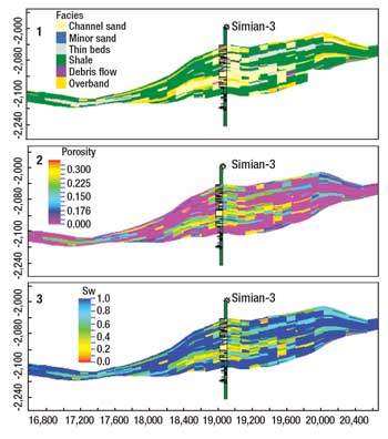
Combining data analysis, with 3D facies models, with the proper trends and variograms produced 3D models of _eff and S_w that represent our approximate view of spatial reservoir property distribution, Fig. 8.

Fig. 8. Three profiles showing in (1) facies model, (2) porosity model and (3) water saturation model.

Horizontal permeability (K_h) was defined based on a function between porosity and permeability extracted from core data and calibrated with DrillStem Tests (DSTs), since DSTs give an approximate measure of actual reservoir permeability. These porosity-permeability equations were generated for both good-quality and poor-quality facies, and then applied in the model. For vertical permeability (K_v), good-quality, deep marine clastic facies had K_v = 0.1 x Kh. But for poor-quality facies (thin beds and debris flows), K_v ranged between 0 and 0.1 x K_h.

UP-SCALING

The process of transferring the data from a fine grid to a coarse grid is called up-scaling. To preserve reservoir heterogeneity, the modelers were required to build the geological grid with relatively fine dimensions (2.4 million cells). But, it wasn’t easy to use the model for reservoir simulation due to the large cell number. Accordingly, another coarser-dimensioned grid was designed. The coarse grid (714,000 cells) was suitable for the dynamic simulation process and preserved essential reservoir details. The concern with it was not only data averaging, but also heterogeneity preservation. The values for _ef, S_w, K_h and K_v were up-scaled using different methods.

Porosity was up-scaled weighted by the bulk volume of the original cells. Since Sw is a function of both bulk volume and pore volume, Sw was weighted by the cells’ pore volume. K_h and K_v are different, since they control the flow of fluids between the adjacent cells. So permeability was up-scaled using a diagonal tensor method.

E-MODEL SELECTION AND VALIDATION

To choose the most representative model from among the six up-scaled models generated, a few validation tests were done. The different models were examined against the original input seismic data and ranked, based on the degree of correlation with the original seismic. The models were then examined against two wells drilled shortly after the model building. Engineering validation depends on testing the up-scaled models dynamically combined with well data and then ranking the models based on that.

Based on the geological/geophysical data and dynamic history matching, the interpreters chose model 6. This model was used for GIIP estimations, predicting well performance, reservoir management and to optimize future development well locations.

IMPROVED INTEGRATED WORKFLOW

Comparing the overall workflow with the standard workflow gives the new workflow added value by combining stochastic and deterministic methods. This advanced usage with multiple scenarios reduced uncertainties within a highly heterogeneous environment. Later testing processes helped improve the degree of model certainty and validity for future actions.

CONCLUSIONS AND RESULTS

Building a 3D reservoir model provides linkage between geological and reservoir engineering disciplines, which share reservoir management. This work helps both disciplines to better understand the reservoir and to make better exploitation decisions. In Simian, understanding the reservoir components, their petrophysical characteristics and their relation with the seismic data as a primary step was a major milestone in the modeling process. It helped to create a live model that acted as a proxy for the actual reservoir.

Grid design was an important step, since an incorrect design could lead to incorrect/less-accurate models. The grid design honored geology and reservoir fluids’ flow direction. The reservoir facies distribution, especially with limited well data, was regarded as the most challenging issue. However, seismic data quality and the modeling approach reduced uncertainties related to spatial facies distribution and provided a solid base for petrophysical modeling.

In models with limited well data, there will be some degree of uncertainty. Ideally, multiple models from different methods are the way to cover most uncertainties. These models can be examined against the geological/engineering data to select the optimum model.  

ACKNOWLEDGEMENTS

The authors thank BG Egypt, Petronas and EGAS for their permission to publish this article. Since reservoir models are teamwork, the authors also thank the team members: Roger Heath, Bahaa Fahmi, Mohamed A. Fattah, Eddi Webb, David Paul and Osama A. Gawad.

LITERATURE CITED

¹ Boucher, J., Dolson, J. and P. Heppard, “Key challenges to realizing full potential in an emerging giant gas province: Nile Delta/Mediterranean offshore, deep water, Egypt,” presented at HGS International Explorationists Dinner Meeting, Sept. 20, 2004.
² Samuel, A., Kneller, B., Raslan, S., Sharp, A. and C. Parsons, “Prolific deep-marine slope channels of the Nile Delta, Egypt,” AAPG Bulletin, Vol. 87, No. 4, 2003, pp. 541-560.
³ Cormac, B and M. John, “Depositional models for the Pliocene submarine channels,” Baker Hughes un-published internal report, 2001.
⁴ Bouma, A. H., “Locations and characteristics of thin bedded turbidites in passive margin setting submarine fans,” Gulf Coast Association of Geological Societies, Vol. XLII, 1992, pp. 425-432.

ADDITIONAL BIBLIOGRAPHY

Brown, A. R., Interpretation of Three-Dimensional Seismic Data, 5th Ed., AAPG, 1999.
Clark, J. D. and K. T. Pickering, Submarine Channels-Processes and Architecture, Vallis Press, London, 1996, pp. 3-18.
Nile Delta & North Sinai Fields, “Discoveries and Hydrocarbon Potentials: A Comprehensive Overview,” Egyptian Petroleum Corporation, Cairo, Egypt, 1994, pp. 3-34.
Posamentier, H. W., “Depositional elements associated with a basin floor channel-levee system: Case study from the Gulf of Mexico,” Marine and Petroleum Geology, Vol. 20, 2003, pp. 677-690.
Roxar, Irap RMS User Guide, release 7.4, 2005.
Said, M., Burley, M. and M. Abdel Fattah, “3D geological reservoir model of Scarab-Saffron: An integrated to slope-channel turbidite modelling,” presented at the Mediterranean Offshore Conference, Alexandria, Egypt, April 20-24, 2004.
Weimer, P. and R. Slatt, Petroleum Systems of Deepwater Settings, 2004, pp.1-1 to 1-15, 2-1 to 2-38, 4-1 to 4-87 and 5-1 to 5-48.