The push is to get into shallow water using techniques different from deepwater electromagnetic methods. Three companies give their unique perspectives.
Perry A. Fischer, Editor
Unlike so many technologies that take decades to catch on, the uptake of electromagnetic technology applied to subsea sediments has been remarkably rapid. The technology is based on the same principles of electrical resistivity that gave rise to the ability to detect hydrocarbons in situ from a wellbore and, arguably, a key in ushering in the modern-day oil field, as well as starting the oilfield services giant Schlumberger. Resistivity is measured from a controlled source that “pumps” electrical energy into the seafloor and is detected at some distance away. Anomalously resistive readings imply a less conductive layer of rock, such as with hydrocarbon-filled pore space.
The uptake has been rapid, both because of the reduction in risk that the technology gives, as well as the luck of having gone commercial at the start of another great boom in high oil prices. But the technology has had difficulty with applications to shallow water. This was not an immediate problem, since the economics of risk reduction in deep water favored those applications. But shallow water was a huge potential market to forego just because of a nagging technical problem.
The problem is the so-called “airwave,” the part of the electromagnetic signal that comes from a towed, controlled source EM generator, goes through the water column and shoots across the water/air interface, as well as the air. This air signal is a major source of unwanted noise that has to be removed. Many solutions have been found-or at least claimed-including separating time from frequency domains, separating the upgoing from the downgoing wave, and the use of transients and multi-transients in step-generated bursts of these partial waveforms.
Which of these works best, and when, is up to the marketplace to determine-and those difficult-to-get case studies will play a key role. Among other things, this article will outline what company is using which method to access the shallow-water EM market, how they are faring, and what their plans are for the near future. Throughout this article, various analogues to seismic will be mentioned-like all analogies, some will be a closer fit than others, and none will be perfect.
IP GRAB
All of the EM companies-Emgs, Ohm, Schlumberger EM, and PGS EM, as well as CGG, have been spending a lot of money in the EM market-and lately for shallow-water EM as well. The prices were high by most measures, perhaps because the stock market has valued all things oily rather high lately. This writer also suspects that it’s driven, in part, by fear that the Intellectual Property will get swallowed up; and if that were to happen, the result would be an uphill legal battle to find yet newer, unpatented methods.
For example, last summer, PGS acquired UK land and shallow-water specialty company MTEM -itself a relative newcomer-while CGG bought a 15% share of Ohm. Meanwhile, Schlumberger bought a “minority interest” in the marine electromagnetics firm PetroMarker six months ago, not long after the company itself was formed. Seafloor-cable seismic specialist RXT made a technology sharing agreement with Houston-based KMS Technologies, but shortly thereafter, Emgs joined with RXT in a 50/50 purchase of all of KMS. This writer does not recall ever seeing a six-month period where competitors invested in so many new companies, all offering very new technologies, especially, shallow-water EM expertise. It is these events that, in part, prompt this article.
THE BUSINESS END
EM is similar to seismic, but it has added some unique wrinkles to the business end, not all of which have been worked out.
What’s in the envelope? The multi-client case. Like seismic, EM data can be acquired for multi-client use. Unlike seismic, the answers it provides tend to be more dramatic. Dave Ridyard, acting president for Emgs Americas, puts it this way: “EM data these days, within their limits, are very accurate. You need an earth model, and if that model matches our measurements, it’s probably right. If the model and the measurements do not match, your model is almost certainly wrong. But, just because the model matches our measurements, doesn’t mean that it’s definitely right. You can still have false negatives and false positives.”
Ridyard continues, “But the probability of a false indicator obviously decreases as data density increases. It’s not a binary DHI-it’s still statistical.”
Leon Walker, president of PGS EM, put it this way: “With seismic, you’re looking primarily at structure; ‘no’ means ‘maybe,’ even with (or without) DHIs, which, in any case, are usually much less definite with seismic than with EM. But with EM, ‘no’ tends to mean ‘no,’ while ‘yes’ means ‘maybe.’”
“So,” Walker continues, “with multi-client EM, the multi-client business can get tricky. Let’s say I have an envelope in my back pocket, and I say to an oil company client, ‘I’ll sell you this envelope for $2 million.’ Let’s say he buys the envelope, opens it, and sees that it’s empty. So then you say, ‘I have another envelope, and I’ll be happy to sell it to you for another $2 million.’ He opens it, and sees that it’s empty, and so on. At least with seismic, there’s always hope and a lot to consider; there’s always a chance. But if [properly modeled] EM data shows no resistors, the chances of finding commercial hydrocarbons are indeed slim, at least within the depth of investigation.”
That depth of investigation varies considerably; it depends a lot on the geology. With seismic, if there are intervening layers that can rob acoustic energy, the depth of investigation shrinks. Similarly, if there are layers of rock/fluid that are shallow and highly conductive, the depth of investigation with EM can shrink.
However, Walker notes that there are places, such as a recent EM acquisition on land in Trinidad, where the geology and structure made seismic imaging lousy, whereas EM, which is often less sensitive to structure, was unaffected. Generally speaking, a depth of 2 km, sometimes 3 km, of subsurface (even deeper under ideal conditions) EM data is usually the most that you can trust nowadays.
The situation is improving all the time, and is very analogous to the state that seismic was in 30 years ago. All of the surface noise, statics, multiples, steep dips and acoustically fast formations that limited the resolution, image quality and useful depth of investigation of seismic have been tremendously improved on. Similar progress should occur with EM over time.
Effect on lease sales. The current shallow investigation limits brings up the odd effect of what will presumably be widespread and routine use of EM data, on land and at sea. Since it strongly tends to give particularly good negative answers in the first kilometer or two of the subsurface, what will be the effect in a country’s lease sales? Although reservoirs might be stacked into shallower depths, they certainly don’t have to be. Will an absence of EM anomalies tend to make oil companies low-grade blocks, resulting in a more thorough look at the shallow subsurface, but at the expense of passing up the deeper, 10-25,000 ft depths? Or will oil companies simply ignore or not buy EM data at all when looking at deeper subsurface targets? No one really knows at this point.
The effect of looking at just the shallower sediments, albeit more accurately, may have other implications. For countries, the effect on lease revenues is hard to predict. It is more likely than not that if nothing anomalous is seen, then the prospectivity will be ranked low, at least in the first 1-3 km where EM can see, and the deeper sediments might not get looked at. On the other hand, with just seismic, the hydrocarbon indicators are generally not as convincing as the EM resistors, so you might go ahead and drill that 15,000-ft well based on structure, sequence stratigraphy, and maybe a hunch. For countries trying to maximize lease sales, EM could have a positive or negative effect on revenues, depending on the luck of whether the first few surveys produce lots of resistive anomalies or very few in the initial rounds. Multi-client EM is in its infancy, and the effect on lease sales could go either way.
As Walker noted, “No doubt, there is a need for a stronger source to improve signal-to-noise.” However, the EM signal depth is not linear with power; rather, it falls off exponentially. So, while higher power does let you see deeper, it follows the law of diminishing returns. Eventually, you run into practical limits due to the generator, the cable and potential environmental effects. So more power will help with investigation depth, but it will still stay relatively shallow. It will probably evolve as another analogy to seismic, where gradual improvement in signal-to-noise will gain at least as much depth as more power.
Shallow economics. In deepwater exploration, the cost of a well can exceed $100 million dollars, which makes it easy to sell EM on the risk reduction of drilling a dry hole. But the economics of shallow water change that equation quickly.
As Ridyard puts it, “Since it’s only looking 2 to 3 km subsurface, and the cost of drilling a relatively shallow well in shallow water could be quite low, it’s a lot harder to say, ‘Would you like us to do a $3 million EM survey to avoid the risk of drilling a $5 million well?’ It’s a question of which shallow water wells are worth spending money to avoid drilling. Now, having said that, we have done shallow-water EM surveys in as little as 60 m, but it’s not an established-market by any means.” It appears that the economics of shallow water EM have yet to be worked out.
PGS uses seafloor cables rather than nodes for its shallow water EM system, which should help the economics. The company has a lot of experience doing seafloor cable work. The cables are designed for use between 20 and 500 m. “Any shallower than that, and the wave action of the transition zone could interfere with our acquisition equipment,” says Walker.
It’s likely that the shallow-water part of the EM business will proceed along a path similar to seismic, where some companies specialize in shallow water and transition zones, while others do not.
THAT PESKY AIRWAVE
As mentioned in the introduction, Controlled Source EM (CSEM) has limitations that have kept applications to deep water, generally due to interference from the airwave, Fig. 1.
 |
|
Fig. 1. The EM source is towed along receiver line at a distance, typically 10 km, before and after first/last seafloor receiver, giving long offsets. Signal travels along subsurface resistive layers but also directly along the water, air/water interface and through the air. Courtesy of Shell E&P.
|
|
Chris Anderson, VP of Global Sales for PGS EM, says that the way forward is to use transients. “Consider a land-based system,” says Anderson. “Instead of a continuous square wave, simply input a step, or transient, function and record what happens at the receiver electrodes some distance away. As soon as the input step occurs, a corresponding instantaneous rise is detected at the receiver due to the propagation (at near light speed) of the electric field through the air. This is followed by the earth response from the subsurface. Current is actually diffusing through the ground along the lines of force set up by the electric field. All the information about subsurface resistivity within the zone of sensitivity, corresponding to that particular offset and position along the line, is contained in that earth step response function,” Fig. 2.
 |
|
Fig. 2. Transient step (partial square wave) at generator (left) and receiver on a land-based system. Airwave is easily discerned from earth response. Courtesy of PGS EM.
|
|
Anderson continues, “The earth’s response is better illustrated by differentiating (plotting the gradient) of the step-response function. The initial step due to the airwave represents infinite gradient, which is followed by the varying gradient of the earth response. The derivative of the step response is the earth’s impulse response function. This function is the key-it contains all the information about the subsurface resistivity. The response starts with a delta-function, or spike, at t = 0, whose strength depends on the surface resistivity. This is the airwave. Represented in this way, it is clear that the airwave precedes the earth impulse response. The airwave is, therefore, clearly separated from the information contained in the earth response. Transient EM systems can therefore operate without interference from the airwave, unlike continuous source CSEM systems,” Fig. 3.
 |
|
Fig. 3. Derivative of the response in Fig. 2. Airwave is clearly separated from earth response. Courtesy of PGS EM.
|
|
“Unfortunately, this is not quite the complete solution. The reason why many CSEM systems use a continuous source is to overcome the very low signal-to-noise conditions that prevail in information from the subsurface due to numerous sources of EM noise. If a transient system is to successfully overcome the airwave issue, it must also address a signal-to-noise problem as well. The solution is to allow a suitable “listening time” after the transient step function has been delivered at the source.
“Electrons must have time to diffuse through the subsurface and the resulting changes in voltage recorded at the receivers. Given this limitation, for a transient system to build signal-to-noise ratio sufficiently to acquire data from deep below the surface, data points must be sampled multiple times to enable data stacking to improve the S/N ratio. The need for stacking data means that there are practical limits in terms of how long it would take to acquire data from more than a few hundred meters below the surface. Clearly, for a transient system to leverage the advantage of airwave separation and be effectively deployed as an alternative to CSEM, signal-to-noise enhancement beyond that provided by stacking data points would be advantageous.
“Fortunately, the task of recovering miniscule signal from overwhelming noise is one that has attracted much research over the years from a number of varying technological applications. One such technique is to use a Pseudo-Random Binary Sequence (PRBS) to drive the switching of the source electrodes in place of a single step function. The proprietary Multi-Transient ElectroMagnetic (MTEM) system employs this technique to overcome the signal-to-noise limitations of transient step functions and is, therefore, able to achieve the necessary airwave separation.
“At the source electrodes, we replace single step functions with a ‘sweep’ of steps achieved by switching the polarity of the source electrodes at varying time intervals controlled by the PRBS. The length of the sweep and frequency of the switching can be parameterized according to the survey objectives. The signal recorded at the receiver now reflects the input signal, and it is no longer immediately apparent that the earth’s impulse response can be determined. To obtain the impulse response with the enhanced S/N ratio, we must deconvolve the source input PRBS signal from that measured at the receiver electrodes. Deconvolution collapses the ‘sweep’ signal into the impulse response we recognize from the derivative of the step response,” Fig 4.
 |
|
Fig. 4. A “sweep” of steps at varying time intervals controlled by PRBS at the input seems to mask the earth impulse at the output (top). Deconvolution of the source input PRBS signal from receiver output restores the earth response but at an improved S/N ratio (bottom). Courtesy of PGS EM.
|
|
“Not only does the technique provide enhanced S/N ratio, but the broad frequency spectrum of the input sequence allows much more rigorous analysis of the returning data. Thus, in addition to the amplitude of the signal being used to measure resistivity, travel time of the earth’s impulse response peak can also be mapped directly to resistivity. Further, the much improved data quality seen in impulse responses derived from this system make full waveform inversion possible.
“In explaining the airwave separation method by which effective S/N ratio is achieved with an MTEM system, the land case was used, which can be thought of as the most extreme case of shallow water. Now recall that in the marine case, the water column suppresses the airwave as water depth increases. For a transient system, where the airwave on land (i.e., with no water column) is perfectly separated from the earth response, the presence of a water column actually serves to smear the airwave into the earth response.
“In the marine case, for a multi-transient system, the recorded impulse contains the earth response that we require with the airwave superimposed. We therefore need a way to remove the influence of the airwave that has been smeared into the record by the presence of the water column. Fortunately, the two components, airwave and earth response, decay at markedly different rates as offset from the source increases.
“Currently, data can be recovered from depths approaching 3,000 m below the seabed by recording data at offsets approaching 10 km. The recorded marine impulse response is a convolution of the earth response, and the response interaction of the airwave with the water column. With long-offset recording, we can separate out the earth response by deconvolving the long-offset airwave record from the marine impulse response, Fig. 5. If, however, we move out to distances approaching 20 km, the signal from the subsurface is so weak as to be negligible and, in this case, we would record only the smeared airwave information.”
 |
|
Fig. 5. By deconvolving the long-offset airwave record from the marine impulse response, we can restore the useful data, but offsets approaching 10 km are the practical S/N limit. Airwave and earth response decay at markedly different rates as offset from the source increases. Useful data can be seen from depths approaching 3,000 m below the seabed. Courtesy of PGS EM.
|
|
World Oil asked Dr. Lucy MacGregor of Ohm for her perspective on shallow-water EM. MacGregor explains, “The traditional view of the airwave signal is that it is a component of the EM field that has traveled up through the water column, through the resistive air at nearly the speed of light, and back to the seafloor, so that in shallow water, this signal, which in theory would contain little information on seafloor structure, swamps the signal through the earth. This view is based largely on a seismic paradigm in which signals can be reduced to rays traveling independently through a medium. Qualitatively, it explains many features of the airwave, but it breaks down in the quantitative analysis needed for detailed interpretation of seafloor CSEM data.”
Dr. MacGregor continues, “Stepping away from this seismic analogy, and considering the true diffusive nature of CSEM fields, you can demonstrate that, in fact, signals that have interacted with the earth and air are tightly coupled; There is no such thing as an ‘airwave’: All signals measured by a receiver depend on both water depth and earth structure. This is equally true in both the frequency domain and the time domain. Moving from frequency to time domain does not change the physics of the situation, and so, signals that are coupled in one, will be equally coupled in the other.”
“In many situations, careful choice of survey design and acquisition parameters, followed by an interpretation using a full-wavefield approach, allows earth structure to be constrained to depths of several kilometers below seafloor despite the shallow water. In other cases, a mode-decomposition approach is required: This can again be applied in either the frequency or time domain, and separates signals into TM mode (relying on vertical current loops) and TE mode (relying on horizontal current loops). The TM mode shows a much smaller dependence on water depth than the TE mode; it is also more sensitive to the thin resistors characteristic of hydrocarbon accumulations, making it an ideal component for probing subsurface structure. Mode decomposition can be accomplished either through acquisition approaches or in post-acquisition processing given appropriate data.
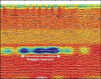
“Ohm conducted the first survey in under 200 m of water in June 2005. This was a proof-of-concept survey on Nuggets Field in the North Sea. Nuggets Field consists of a 20-m-thick gas sand at a depth of about 1,700 m below the seafloor, in 116-m water depth. The results were extremely positive.” The resulting inversion of the data, using structural constraints from seismic data, is shown in Fig. 6-the gas sand is clearly imaged as a high-resistivity (blue) area.
 |
|
Fig. 6. The high resistor is a gas-sand reservoir; data acquired in 200 m water depth. Courtesy of Ohm.
|
|
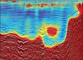
Dr. MacGregor continues: “Since the first proof-of-concept survey, we have gone on to survey numerous reservoirs and potential reservoirs in water depths less than 300 m. For example, in January 2006, we performed a survey on the Ernest prospect in the North Falkland Basin. The survey aimed to de-risk the prospect by confirming the presence (or absence) of resistive strata in the prospect area. Not only was this a shallow-water survey done in ~160 m deep water, but the interpretation was further complicated by the proximity of the prospect to resistive faulted basement. Results were again positive, with a localized resistive zone imaged coincident with the seismically defined structural closure,” Fig. 7.
 |
|
Fig. 7. Shallow-water (~160 m deep) survey, complicated by proximity to resistive faulted basement. Results show a localized resistive zone coincident with seismically defined structural closure. Courtesy of Ohm.
|
|
“We routinely operate in shallow water without problem-indeed, a large proportion of surveys conducted by us in the last year have been in less than 300 m of water, with the shallowest survey to date conducted in 30 m of water last summer. We are in the process of planning a survey in 10 m of water. Water depth is no longer a constraint for us. Surveys in all water depths (or rapidly varying water depth) are possible, providing sufficient care is taken in the pre-survey planning and post-survey interpretation.”
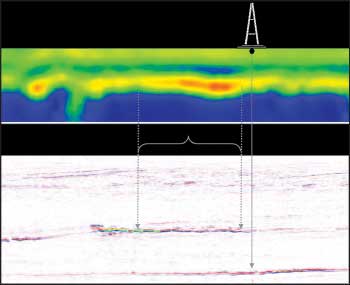
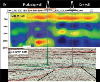
Anderson with PGS EM describes his company’s success. “The multi-transient, PRBS-sweep, EM method provides the airwave separation and has addressed the S/N ratio issues. 2D resistivity profiles acquired, processed and inverted from the MTEM system have produced encouraging results from the North Sea, where prospects have been identified at depths ranging from 900 m down to 2,200 m. These have been acquired in as little as 100 m of water depth. Data from Apache and BP Harding correlate well,” Fig. 8.
 |
|
Fig. 8. Seismic section below shallow EM data show good correlation with a known North Sea reservoir. Courtesy of PGS EM.
|
|
IS TRANSISTION THE SAME AS SEISMIC?
Sometimes with seismic, the equipment and methods have to be changed as the water becomes shallow. Does that happen with EM? Dave Ridyard with Emgs talked about transition from shallow to deep water: “Even before we purchased KMS, we were well along in the use of continuous-source CSEM for shallow waters. We used existing methods such as upgoing/downgoing wave separation, which have been discussed in the literature since about 2000. As I mentioned before, we’ve done a commercial survey in as little as 60 m of water. Fortunately, our equipment is able to switch between continuous and transient modes without removing it from the water. For practical purposes of time and productivity, if you were doing a very shallow-to-deep survey, it would probably be best to keep your vessel speed up and make two passes, one in each mode, rather than switch back and forth at a lower vessel speed.”
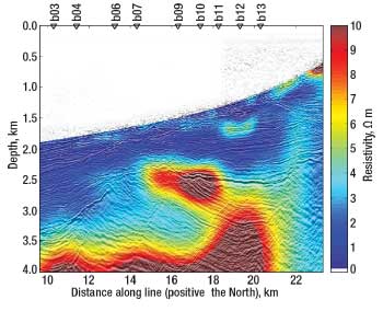
Dr. MacGregor explains Ohm’s approach. “In many exploration situations, the water depth varies from deep to shallow water along the survey line. For example, we conducted a survey for CNR in 2006 across Baobab Field in Cote d’Ivoire. The water depth varied from 2.2 km at one end of the line to 200 m at the other end. The resulting dataset could therefore be termed a hybrid.
To interpret a dataset of this sort, in which the water depth varies so dramatically along a line, the variation in signal interaction with the air must be carefully accounted for in the inversion process. This is done by using an unstructured finite element mesh to accurately model the fields as the water depth changes, thereby taking the variation in signal interaction with the air into account in the inversion process.” The Baobab Field line is shown in Fig. 9.
 |
|
Fig. 9. The result of unconstrained inversion of Baobab Field data, co-rendered with coincident seismic data. Despite the dramatic variation in water depth, the reservoir is accurately imaged. Courtesy of Ohm.
|
|
THE ROAD AHEAD
Like other geophysical disciplines, different companies take different approaches. Ridyard says, “Transient EM is a part of cracking the shallow-water problem. Although we have not done a fully commercial transient EM project yet, there are methods other than transient. We also recently used our new 3D inversion method, which, combined with up/down separation, is potentially another way to crack the shallow-water problem. So our approach is that we acquire a toolkit, if you will, where we can use transients, up/down separation and other techniques depending on how the area tests and choose one that works best for both acquisition and processing.”
Anderson notes that his company’s current shallow-water dual-vessel system is designed to operate with an ocean bottom cable linking up to 40 pairs of receiver electrodes, and static dipole source. “Maximum water depth is limited only by the design specifications of the cable, which is 500 m. Maximum penetration depth depends on a number of factors, but is considered feasible down to 3,000 m below the seabed. However, future developments will include a more powerful source that will extend the penetration depth and reduce acquisition time.”
Anderson adds, “The ability to measure subsurface resistivity from the surface in the most productive areas of the world has opened up the possibility of integrating EM data into reservoir management workflow. The resolution that can be achieved using multi-transients in shallow seas and onshore means that EM data can now be incorporated into the decision process of extensive drilling programs, improving success rates, extending and enhancing production in areas close to existing markets and infrastructure. This is an area that has, until now, not benefited from the application of the new generation of EM techniques.”
Finally, it should be mentioned that PGS has been working for the past four years on a continuous streamer-towed EM system, having conducted at least two tests in the North Sea. While the technical difficulties are considerable, the company remains optimistic and will continue work on the technique, considering the benefit in productivity/costs compared to a node receiver system.
Dr. MacGregor describes the possibilities: “CSEM surveys help clients de-risk exploration prospects. However, the technique also has applications in reservoir appraisal and management. We have an ongoing R&D project, funded by the UK government and working in collaboration with BP, to develop these applications. One of the key components of moving from an exploration to a production environment is the intelligent integration of CSEM data with complementary data from seismic and well logs. By doing this, we can use the strengths of each to move beyond simple images of resistive and conductive structure, and provide maps of lithology and fluid properties across a field.”
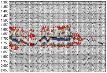
An example from the shallow-water Nuggets Field (~120 m) is shown in Fig. 10. “Working with Rock Solid Images, we were able to integrate the CSEM data with coincident seismic data, calibrated to well-log information, to produce a semi-quantitative map of gas saturation across the extent of Nuggets Field.
 |
|
Fig. 10. The potential for reservoir management: An example from the shallow-water Nuggets Field that integrates (superimposes) CSEM data with seismic and well-log data, to produce a semi-quantitative map of gas saturation across the field. Blue is high gas saturation, red is low. Courtesy of Ohm.
|
|
“Although this is a simple example, it demonstrates that by integrating geophysical data types we can provide information on a reservoir that is either not available or is unreliable using any one data type alone. By doing this, we hope to improve the quality of reservoir information available to engineers and geoscientists making decisions on field development and management in the future.”
A FINAL WORD
The last analogy with seismic that this writer will make is simply this: Seismic took many decades to get to the 3D/4D, AVO/DHI state of the art that we know today, and it’s made an extraordinary contribution to finding oil and gas. EM as an exploration tool, in all its forms, will make at least as great a contribution to the world, and it won’t take as long. 
ACKNOWLEDGMENT
The author is grateful to the following people for their time, without which this would not have been possible: Dr. Lucy MacGregor with Ohm; Jason Tinder with Rock Solid Images; Chris Anderson, Leon Walker and John Walsh with PGS; and Dave Ridyard and Carl Hutchins with Emgs.
|

