After more than four years of use, 3C land seismic has proven itself worth the cost and effort, as it makes for better well placement and production.
Paul F. Anderson, Apache Canada Ltd.
In 2004, Apache began investigating the use of multi-component technology. One of the projects initiated was to target upper-Mannville channel sands to discriminate gas-charged porosity. Several papers have been published reviewing the acquisition design, initial processing and interpretation.1-4 Additional efforts have been put toward the analysis in the past few years in order to better utilize the multi-component data recorded. The data were used to generate a Joint PP-PS prestack inversion, which was then incorporated into a neural networks analysis for further lithology discrimination. The vertical and horizontal components of the PS data were also analyzed for shear-wave splitting to detect anisotropy.
INTRODUCTION
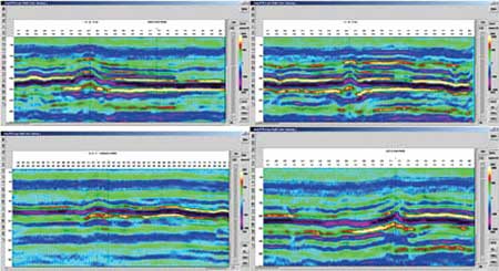
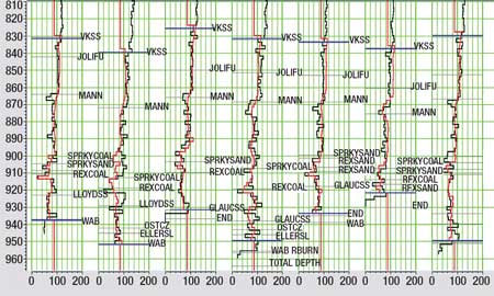
Before utilizing the converted wave seismic data, these channels were identified using the residual PP-time structure from conventional 3D seismic data. The first development phases focused on drilling those anomalies with the most residual structure. The well results indicated a more complicated stratigraphic scenario, Fig. 1.
 |
|
Fig. 1. P-wave structure alone cannot identify good drilling locations. Good gas wells with good structure are shown in (a) and (d). A dry hole was drilled into the good structure shown in (b) and a productive well was also drilled into a location with moderate structure (c).
|
|
The multi-component data was evaluated to determine if the converted wave amplitudes were indicative of the lithology within the channel (i.e., reservoir vs. non-reservoir). The preliminary interpretation showed variations in the PS amplitude along the channel trend defined by the PP-time structure map, which were compared to well results.3
This article investigates using multi-component data as input into an inversion process and as an attribute for neural network analysis. To assess the results, the joint inversion incorporating the converted wave data was compared to two other common inversion methods, post-stack inversion of AVO attributes5 and prestack inversion of angle stacks.6
POST-STACK INVERSION OF P-WAVE AVO ATTRIBUTES
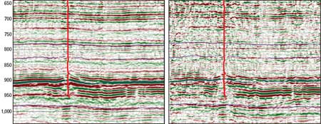
The process of estimating rock properties with a post-stack inversion method follows the procedure outlined by Goodway et al.5 Additional processing was applied to the gathers to help improve the signal-to-noise ratio. An angle range of 5°−30° was used for the AVO inversion as the near offsets are subject to acquisition artifacts, while the larger angles exhibit issues due to anisotropy. Upon extraction of the AVO attribute volumes, post-stack inversion was performed. Cross-sections taken from the P-wave and S-wave reflectivities are shown in Fig. 2. The AVO inversion of prestack P-wave seismic gathers generates P-wave reflectivity and S-wave reflectivity. Using well log information, background P- and S-wave impedance models can be built, which are then used to invert the corresponding AVO attributes following standard practices for post-stack impedance inversion. After the inversions have been completed, calculation of rock properties is a simple matter of trace math.
 |
|
Fig. 2. AVO attributes Rp (left) and Rs (right). The sonic log from Well F is shown as the red line in the displays. The zone of interest is at about 925 ms.
|
|
PRESTACK INVERSION OF P-WAVE SEISMIC DATA
The procedure for prestack inversion of P-wave seismic data followed the workflow presented by Hampson et al.6 The concept is intended to arrive at the same point as the workflow provided above, using fewer steps and in a more integrated fashion. By performing the inversion prestack, P-wave impedance and S-wave impedances are solved for simultaneously, thereby treating errors equally on both volumes. We are also able to account for wavelet variability from near to far angles by inverting using multiple wavelets.
The background model used for the post-stack inversions was also used for the prestack inversions, in order to maintain consistency for comparison. To account for frequency content differences from near to far angles (frequency content changes can occur with offset due to a variety of reasons, including transmission effects and NMO-stretch), near angle (5°) and far angle (25°) wavelets were extracted. These wavelets were extracted using Roy White’s algorithm for wavelet estimation to account for frequency-dependant amplitude and phase variations that may exist in the data. The Vp/Vs calculated using this method is shown in Fig. 3.
 |
|
Fig. 3. Vp/Vs calculated from inversion of P-impedance and S-impedance from prestack inversion.
|
|
PRESTACK INVERSION OF P-WAVE AND CONVERTED WAVE SEISMIC
Integration of the converted wave data to the inversion follows a similar path as previously defined for the PP-only prestack inversion above. Using the same P-wave angle gathers created for the previous inversion, converted wave data is also included. Before incorporating the converted wave information, however, this data must first be registered to P-wave time. Registration is performed using two geologic events and correlating these in time using a method similar to manual well-ties, similar in many ways to performing a depth conversion of seismic data in two-way time.
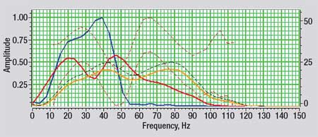
After registration, a wavelet is also required for the converted wave data in order to include it in the inversion. Figure 4 shows a comparison between the three extracted wavelets, PP-near (orange), PP-far (red) and PS-registered (blue). We note immediately that even after registration, which compresses the converted wave data, the converted wave data remains of lower frequency than the P-wave data. One reason for this is strong anisotropy, which is discussed later.
 |
|
Fig. 4. Near (orange) and far (red) angle wavelets from P-wave data compared to the converted wave wavelet (blue) used in joint prestack inversion. Note that the converted wave wavelet has significantly lower bandwidth than either P-wave wavelet.
|
|
DISCUSSION
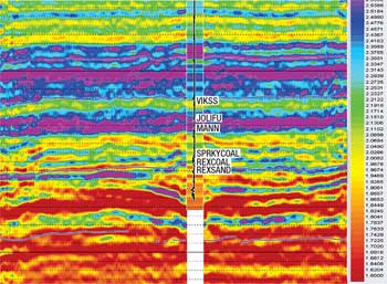
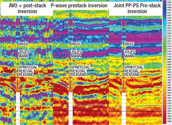
Figure 5 shows a comparison of the three different Vp/Vs estimates, each using the methods described above, for the same cross-line. Inserted into each section is the Vp/Vs calculated from depth-time relationships, derived from well-ties, for comparison.
The three sections shown in Fig. 5 all have different frequency content, from high, using the method proposed by Goodway, to low, when incorporating the converted wave data in the inversion. It is believed that the very high frequency content of the AVO plus post-stack inversion is due to noise created in the inversion process. Because the impedance volumes were decoupled in their calculation, bed-boundaries were calculated as occurring at slightly different time-samples for each trace, resulting in a high-frequency jitter being introduced from the misalignment of the combined volumes.
 |
|
Fig. 5. Comparison of Vp/Vs is calculated from AVO plus: post-stack inversion (left), prestack inversion (middle) and joint prestack inversion (right). Vp/Vs from logs at Well D have been inserted in color and the SP log as the trace.
|
|
Note that the prestack joint inversion appears to have significantly lower frequency content than either of the other two methods, especially above the zone of interest. One possible explanation is that the registration process has caused the wavelet on the registered converted wave data to become non-stationary in time (and possibly space), violating a key assumption of our inversion. This result comes from different portions of each converted wave trace being compressed a different amount, depending upon the Vp/Vs used for registration.
All three methods generate Vp/Vs volumes that match log response reasonably well, with the general exception of the coals. The limitation here comes from the assumption in the Aki and Richards approximation7 to the Knott-Zoeppritz equations, where it is assumed that reflectivity contrasts are relatively small, i.e.,
This assumption plays a role in all three inversion methods mentioned above. Because the impedance contrast of the coals immediately above the zone of interest is about 10 times higher than the average background reflectivity, this assumption is violated and the solution at that level has large inherent errors.
Based upon the results presented here, prestack inversion, used alone or with converted wave data, appears to be the best methods to estimate Vp/Vs from seismic data; however, this conclusion is based upon qualitative results to date only and quantitative comparison is currently in progress.
NEURAL NETWORK ANALYSIS
The use of neural networks to calculate well log properties has been well documented over the past several years.8,9 The attribute volumes generated from the converted-wave data can be included in the process to add one more dimension to the analysis.
One of the potential advantages to using neural networks is that it may be possible to account for small-scale registration issued between the P-wave and converted wave data, as we can make use of a multi-sample operator to perform the analysis. Provided that the registration error is stationary, a refined registration is effectively built into the procedure.
With all seismic data volumes, the number of attributes available to the interpreter can become staggering. Neural networks allow an interpreter to distill all available information from multiple attributes, potentially numbering into the hundreds, into a single attribute. In this case, we have more than 20 attributes that have been calculated from the seismic data, encompassing the various AVO and inversion products discussed, in addition to derivative attributes (e.g., LMR). In this case, we are estimating gamma ray to be used as a first-pass, reservoir-quality indicator.
The first step in the process is to train the network at well locations. This determines the processes that need to be applied to the seismic attributes to derive the best estimate of gamma ray at the wells. Through this step, a number of parameters are selected, including:
- Length of the convolutional operator used in network
- Combination of attributes to use
- Optimum number of attributes to use.
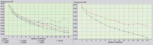
All of these are selected to minimize the validation error in the estimate. Figure 6 shows a validation plot of the number of attributes versus RMS error in the estimate. The various curves plotted are for different operator lengths. In this case, we can see that the error is minimized using a five-point operator with 11 attributes. Despite the problems that remain in the data for the joint prestack inversion, three of the attributes used in the gamma ray prediction came directly from converted wave data, one attribute even being the Vp/Vs from the joint inversion.
 |
|
Fig. 6. Left image shows a comparison of the number of attributes versus the validation error for a range of operator lengths. The lowest errors are seen on the blue curve using 11 attributes. Over-training of the network is visible by comparing the validation error (red) to the training error (black). Where the curves begin to diverge defines the point at which additional attributes serve only to over-train the network.
|
|
It is important to not simply apply the results, but to validate the results by leaving out wells, one at a time, and rerunning the process to ensure that the neural network is not over-trained. This occurs when the fitting of the attributes to the wells is so precise that it is no longer able to predict additional wells added to the analysis, making the results away from the wells invalid. The list of specific attributes used to train the neural network is provided in Table 1. This list of attributes, derived from multi-linear regression, is then used to refine the estimate using a neural network, which allows for non-linear transforms of the data to improve the results.
| TABLE 1. Neutral netword attributes |
 |
|
In examining the residual errors in estimating the gamma ray log from seismic data, we have a correlation of about 81% to the real gamma ray logs and an RMS error of 12 API units. A comparison of the real (black) and predicted (red) gamma ray logs is shown in Fig. 7. For each well, we see relatively high correlations between the predicted and actual gamma ray responses, with an average correlation of approximately 81%, which corresponds to an error of 12.4-API units averaged over all 12 wells.
 |
|
Fig. 7. Comparison of the actual and predicted gamma ray logs at 7 wells. Each block corresponds to 2 ms in two-way-time.
|
|
Given that the size of each block in this display corresponds to 2 ms, the level of detail achieved through this technique is excellent. Some disconnects still exist near the coals; however, this may be due to the small reflectivity assumption already discussed.
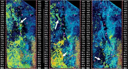
Now that the neural network has been trained, we can apply the results to the full seismic volume and calculate a predicted gamma ray trace for every CMP. Figure 8 shows a comparison between the predicted gamma ray cube at the coals, and at three different horizon slices through the channel. Arrows indicate where apparently new information can be gleaned from this new attribute about reservoir quality. In the left image, for example, a well is indicated which had no production, though it was drilled into the center of the channel. The predicted gamma ray cube shows that cleaner reservoir sands may be present on the edges of the channel. An undrilled, but isolated low-gamma ray region is identified to the north in the center image, along with previously unidentified channel-like features to the south, also visible in the right image.
 |
|
Fig. 8. Slices through the predicted gamma ray cube at various levels through the channel. Additional detail, not previously seen on seismic data, is now visible, indicating different reservoir quality both within and outside the main channel body, identified by the north-south pattern of wells through the middle of the images.
|
|
FURTHER APPLICATIONS
As discussed above, the frequency content of the converted wave data, even after registration, is significantly lower than the conventional P-wave data. One of the causes for this is the presence of anisotropy, which has not yet been accounted for in processing. While the effects of anisotropy are present on P-wave data, they have a much stronger impact on the converted wave data, due to longer travel times. Despite the fact that anisotropy causes problems on the converted-wave data, the look-back performed earlier showed that the converted wave data, in its current state, has been deemed useful in providing reservoir information.
Theory predicts as shear waves propagate through an anisotropic medium, for example, a thick coal with cleats, the shear waves (Sv and Sh) become polarized in the direction of the cleats, resulting in time delays that are dependent upon azimuth for a particular CCP gather. When it is present, this time-delay can appear to be residual statics or velocity errors on the radial data. It also results in residual, coherent energy on the transverse component. If present, some of the amplitude variations we see in the converted wave data may be related more to anisotropy of shallower layers of rock instead of what is typically attributed to AVO.
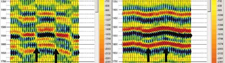
Rotation analysis of the radial and transverse data was performed to evaluate the presence of shear-wave splitting. Upon investigation of the transverse component, residual coherent energy was found, so PS1-PS2 rotation analysis was performed at a few select locations for further analysis. Figure 9 shows a sample CCP gather radial and transverse components for this rotation analysis.
 |
|
Fig. 9. Cross-section of PS data for the transverse (left) component and radial (right) component at a single CCP location for different rotations. Note that the azimuths of the polarity reversal on the transverse component match to the fast (PS1) and slow (PS2) orientations of the shear waves.3
|
|
The transverse component shows characteristic polarity reversals which correspond to the fast and slow shear wave azimuths. By examining the radial component we can determine that the fast shear is oriented 55° E of N and the slow is perpendicular to that at 35° E of S. The radial data shows a time delay of approximately 13 ms down to the top Mannville; however, when measuring the time delay at the Rex Coal, it is about 17 ms, indicating an increase in anisotropy within the upper Mannville, above the Rex coal. Other locations investigated seem to indicate that both the magnitude and direction of the anisotropy changes in all three dimensions. As a result, many of the amplitude changes we are seeing on the converted wave data may not be related to changes in rock properties at the reservoir, but changes in anisotropy above the reservoir. Correctly processing for this effect will not only improve the event continuity of the converted wave data, but also improve the frequency content by removing what effectively amounts to a spatially and depth-dependent static.
CONCLUSIONS
To this point in the process, a great deal has been learned about the potential value of 3D converted wave seismic data, in the context of identification of reservoir sands. Based on the work shown here and in previous publications, the following is a summary of what we have learned:
- P-wave structure combined with converted wave amplitude can raise the success rate for these Mannville-age channels, and can be done quickly with conventional interpretation tools.3
- Shear-wave anisotropy is a critical component to consider when dealing with converted-wave data, even in an unstructured environment.10
- Joint prestack inversion of conventional and converted wave seismic data can be performed to estimate rock properties.
- Additional attributes from converted-wave data can be included in neural network analysis. Solving for one attribute, e.g., gamma ray, provides a volume for lithology discrimination.
While this study has been underway, additional drilling has continued in the area. A critical step still missing from this process is to compare the new drilling results against the various attributes described herein, especially the gamma ray cube, to determine the true reliability of the results. Additionally, further improvements to the conventional and inverted wave data, by accounting for anisotropy in the processing, are expected to yield a number of critical improvements, including:
Improved frequency content of the converted wave data
- Improved amplitude consistency
- Improved resolution for registration, allowing for events to be better aligned in the inversion process.
Additional attributes can be included in the neural network analysis that have interpretive significance (e.g., magnitude of anisotropy and orientation). 
ACKNOWLEDGEMENTS
Special thanks to Apache Corporation and VGS Seismic for permission to publish this work. Thanks also go to Ron Larson, Dave Monk, Glenn Murdock, Buzzy Mitchell and Craig Rice of Apache; Graham Carter, Janusz Peron and Keith Hirsche of CGGVeritas Hampson-Russell; and Larry Lines, Rob Stewart and John Bancroft from the CREWES project at the University of Calgary for their technical assistance and insights. Thanks also go to Heather Joy, Apache, for her review and input to this article.
LITERATURE CITED
1 Monk, D., Larson, R. and P. Anderson, “An east-central Alberta multi-component seismic case history,” Recorder, Vol. 31, pp. 18−22, 2006.
2 Roth, M., “Practical interpretation of multi-component seismic data,” Recorder, Vol. 31, pp. 23−26, 2006.
3 Anderson, P. F. and R. Larson, “Multi-component case study - One company’s experience in Eastern Alberta,” Recorder, Vol. 31, p. 510, 2006.
4 Anderson, P. F., “Multi-component case study - continued multi-component experience in eastern Alberta,” 77th Annual International Meeting, SEG, Expanded Abstracts, 2007.
5 Goodway, B., Chen, T. and J. Downton, “Improved AVO fluid detection and lithology discrimination using lame petrophysical parameters, fluid stack from P and S inversions,” 67th Annual International Meeting, Soc. of Expl. Geophys., pp. 183-186, 1997.
6 Hampson, D. P., Russell, B. H. and B. Bankhead, “Simultaneous inversion of pre-stack seismic data,” 75th Annual International Meeting, SEG, Expanded Abstracts, pp. 1,633-1,637, 2005.
7 Aki, K. and P. G. Richards, Quantitative Seismology, Vol. 1, Sec 5.2, 1980.
8 Herrera, V. M., Russell, B. and A. Flores, “Interpreter’s corner - Neural networks in reservoir characterization,” The Leading Edge, Vol. pp. 25, 402-413, 2006.
9 Anderson, P. F., Chabot, L. and D. Gray, “A proposed workflow for reservoir characterization using multi-component seismic data,” 75th Annual International Meeting, SEG, Expanded Abstracts, pp. 991-994, 2005.
10 Anderson, P.F. and L. Lines, “A comparison of inversion techniques to predict Vp/Vs from 3D seismic data,” CREWES Annual Report, 2008.
ADDITIONAL REFERENCES
Fatti, J. L. et al, “Detection of gas in sandstone reservoirs using AVO analysis: A 3-D seismic case history using the Geostack technique,” Geophysics, Vol. 59, pp. 1362−1376, 1994.
Gaiser, J., 1999, enhanced PS-wave images and attributes using prestack azimuthal processing. 69th Ann. Internat. Mtg: Soc. Of Expl. Geophys., 699-702.
Gidlow, P. M., Smith, G. C. and P. J. Vail, “Hydrocarbon detection using fluid factor traces, a case study: How useful is AVO analysis?” Joint SEG/EAEG summer research workshop, Technical Program and Abstracts, pp. 78−89, 1992.
Ostrander, W. J., “Plane-wave reflection coefficients for gas sands at nonnormal angles-of-incidence,” Geophysics, Vol. 49, No. 10, pp. 1637−1648, 1984.
White, R.E., 1997, “The accuracy of well ties: practical procedures and examples,” presented at the 1997 SEG Annual International Meeting, Expanded Abstracts, Vol 2, RC1.5, 2126.
|
THE AUTHOR
|
|
|
Paul Anderson earned a BSc degree in geophysics from the University of Calgary and is a geophysicist in the Exploration & Production Technology group at Apache Canada Ltd. Paul’s responsibilities include advising on seismic processing, AVO analysis, inversion, converted wave analysis, VSP data and microseismic. Before joining Apache in January 2006, Paul was with Veritas GeoServices in Calgary and Houston, where he was responsible for AVO, AVAZ, inversion, converted wave interpretation and rock properties analysis. He has experience in a number of geologic basins, including Western Canadian, the Canadian East Coast, Beaufort Sea and Mackenzie Delta, Gulf of Mexico, onshore Texas, offshore Brazil, onshore Egypt and offshore Australia. Currently Paul is working on his master’s degree with the CREWES project at the University of Calgary and is a member of APEGGA, CSEG, CSPG and SEG.
|
|


