Reservoir Characterization

Pore pressure in the Gulf of Mexico: Seeing ahead of the bit

A pore pressure cube built over the entire northern Gulf of Mexico using data released by the Minerals Management Service (MMS) substantially reduces the time needed for pore pressure prediction projects in this area. Data acquired while drilling allows the pore pressure prediction ahead of the bit to be improved and the uncertainty to be reduced.

Colin Sayers, Lennert den Boer, Zsolt Nagy, Patrick Hooyman, and Victor Ward, Schlumberger, Houston

Knowing pore pressure is becoming increasingly essential for drilling in depleted, deep or overpressured zones. Pre-drill, pore pressure can be predicted using fit-for-purpose seismic velocities with a velocity-to-pore pressure transform calibrated to offset wells. To reduce the time required for such projects, it was decided to build a pore pressure cube over the entire northern Gulf of Mexico, using data released by the Minerals Management Service (MMS). This paper describes the workflow used to build the regional, northern Gulf of Mexico pore pressure cube.

All released checkshots for the Gulf of Mexico were inverted for velocity versus depth below mudline, then kriged to populate a 3D Mechanical Earth Model (MEM) with both velocity and expected uncertainty. The 3D velocity cube thus obtained was used to infer regional variations in overpressure. Once an area of interest for drilling has been identified, any extra data provided by the client can be added to increase the local model resolution. This refinement process continues with data acquired while drilling, which allows the uncertainty in pore pressure prediction ahead of the bit to be reduced ahead of the drill-bit.

INTRODUCTION

Pore pressure can be predicted from seismic velocities via a velocity-to-pore pressure transform calibrated to offset wells, Fig. 1, where pore pressure in the GOM, predicted from reflection tomographic seismic velocities¹, is overlain on the migrated seismic volume.

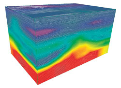Fig. 1. Pore pressure prediction in the Gulf of Mexico using seismic velocities from reflection tomography, with a velocity-to-pore-pressure transform calibrated to offset wells.1

This approach has recently been extended to include an estimate of pore pressure uncertainty, using Monte-Carlo methods to build a 3D probabilistic mechanical earth model.² The technique employs a velocity-to-pore pressure transform based on a rock physics analysis of available offset wells.³ An example of a pore pressure prediction using this method is shown in Fig. 2, while Fig. 3 illustrates how the resulting model can be used for well planning.

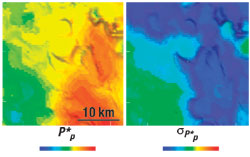Fig. 2. Pore pressure (left) with uncertainty (right) predicted using a probabilistic mechanical earth model, or P-MEM2 with a velocity-to-pore pressure transform based on a rock physics analysis of offset wells.3

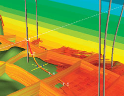Fig. 3. Use of a probabilistic mechanical earth model for well planning.2

Pore pressure studies like those shown in Figs. 1 – 3 typically take 1 – 2 months to perform, whereas drillers often require a faster result. To reduce the time required, a pore pressure cube was built covering the entire northern GOM, using data released by the MMS. All checkshots released by the MMS in the Gulf of Mexico were inverted to obtain compressional velocity versus depth below mudline. These velocity functions were then kriged to populate a 3D MEM with both velocity and expected uncertainty. The 3D velocity cube thus obtained was used to infer the regional variation in overpressure and undercompaction of shallow sediments.

By applying a threshold to the predicted kriging error, maps of undercompaction and overpressure can be limited to areas of greater reliability. The methods developed and presented here should find wide application in the drilling of safe and economic wells in overpressured regions.

VELOCITY SENSITIVITY TO UNDERCOMPACTION

In the GOM, compaction disequilibrium is the most important cause of overpressure. For sediment to compact, pore water must be expelled. However, if sedimentation is rapid compared to the time required for fluid to be expelled from the pore space, or if seals that prevent dewatering and compaction form during burial, the pore fluid becomes overpressured and supports part of the overburden load.

Elastic wave velocities in rocks normally increase during loading due to porosity reduction and increased grain contact. Because of overpressure, the porosity is higher and the elastic wave velocity is lower than in normally pressured sediments. This situation is illustrated in Fig. 4, where (for illustration) the increase in velocity with depth below the mudline is represented by a linear depth gradient k:

Fig. 4. Schematic variation of elastic wave velocity with depth below mudline for normally compacted and undercompacted sediments.

In areas undergoing rapid sedimentation, the compaction coefficient k is smaller than in areas of slower sedimentation, where pore pressures induced by loading have sufficient time to dissipate. Overpressures resulting from compaction disequilibrium can therefore be predicted, given sufficiently accurate seismic velocities.⁴ Velocities employed for this study were obtained by inversion of checkshot data released by the MMS for the GOM.

CHECKSHOT INVERSION

Fig. 5 shows the locations of checkshots included in the study, corresponding to all the surveys available from the MMS archive at the end of 2004. Fig. 6 shows time-depth pairs from a typical checkshot survey, together with interval velocity calculated from the relation:

Fig. 5. Locations of checkshots (red dots) currently released by the MMS in the Gulf of Mexico, relative to the coastline (blue).

Fig. 6. Time-depth pairs for a checkshot in the GOM (left), together with interval velocity calculated as the difference in depth divided by the difference in time for adjacent receiver positions (right).

From Fig. 6, it is evident that the velocity versus depth profile is adversely affected by picking errors in the measured travel time. Accordingly, a weighted damped least-squares inversion of the measured travel times was employed to compute velocity-depth profiles consistent with the errors in the travel time data.

Following Lizarralde and Swift⁵, the interval velocities between receivers may be determined from measured first arrival times, by solving the linear equation:

where t_i are the first-arrival times at each receiver depth (i=1..N),Dz_i are difference in depths between receivers, and s_i = 1/v_i are the interval slownesses, v_i being the interval velocities. It is convenient to write Eq. 3 as

A damped least-squares inversion was performed⁵, employing a penalty function based on the second derivative of estimated slowness as a smoothing criterion. A least-squares solution was obtained by minimizing:

where || || denotes the L₂ norm, D is the second-derivative matrix, DS is the penalty function, and Î is the damping parameter, governing the trade-off between minimization of the data misfit and the penalty function. Fig. 7 shows the inverted interval velocity as a function of depth for several values of Î. An appropriate choice of Î was made by examining the associated travel time residuals.

Fig. 7. Damped least-squares inversion of a checkshot (Fig. 6) for various values of Î in Eq. 5.

CONSTRUCTION OF THE 3D VELOCITY MODEL

Following inversion of the checkshots, the derived interval velocity versus depth profiles were loaded into a 3D geostatistical modeling application, together with sonic and density logs from several deepwater wells released by the MMS. A detailed sea-bottom surface for the entire western GOM (15-sec. resolution) was derived from bathymetry and elevation data (NGDC) for the geographical region between – 83° to – 97° longitude, and 26° to 30° latitude, Fig. 8.

Fig. 8. Water bottom depth (ft subsea).

A 3D curvilinear stratigraphic grid was constructed conformable to this mudline surface by spline interpolation, to a maximum depth of 30,000 ft subsea. Each cell in the stratigraphic grid measures 0.05° × 0.05° in area (about 3.5 × 3.5 sq mi, or one block), by 60-ft thick. A 3D estimate of bulk density was derived using a relation of the form given by Traugott⁶, calibrated to available deepwater density logs. Density was then integrated to obtain overburden stress. A corresponding 3D velocity trend was obtained from density via Gardner’s relation, calibrated to available sonic logs.

After upscaling to the stratigraphic grid, the combined checkshot and sonic velocities were kriged, using the 3D velocity trend as an estimate of the local mean in each cell, assuming an exponential model of spatial correlation with a laterally isotropic effective range of order 1°, and vertical range of order 600 ft. The resulting trend-kriged velocity model is shown in Fig. 9, with the 3D distribution limited to a region where the average predicted kriging error (Fig. 10) is less than ±1,200 ft/sec. Fig. 11 shows a map of the compaction coefficient k draped on the water-bottom surface, also limited to the area where velocity error is less than 1,200 ft/sec. This map was obtained by minimizing the rms difference between kriged velocity and Eq. 1 for the first 10,000 ft below mudline. The compaction coefficient thus obtained is seen to be minimum in the deepwater areas near the shelf edge, indicating that undercompaction is greatest in this region.

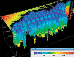Fig. 9. Velocity model (in ft/sec) obtained by trend kriging inverted checkshots and sonic logs from deepwater wells released by MMS, for all locations where the predicted kriging error (Fig. 10) is less than ±1,200 ft/sec. (Scale for land elevation above sea level is not shown).

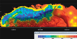Fig. 10. Average predicted kriging error (ft/sec) for trend-kriged inverted checkshots and sonic logs from deepwater wells released by MMS, draped on the water-bottom surface.

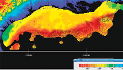Fig. 11. Map of compaction coefficient k (sec-1) derived by minimizing the rms difference between Eq. 1 and trend-kriged velocity (Fig. 9), for all locations where predicted kriging error (Fig. 10) is less than ±1,200 ft/sec. (Scale for land elevation above sea level is not shown).

PORE PRESSURE PREDICTION

Since any increase in pore pressure above the normal hydrostatic gradient reduces the amount of compaction that can occur, elastic wave velocities can be used to predict pore pressure. This was first demonstrated⁷ using sonic velocities. In the following discussion, it is assumed that elastic wave velocity is a function only of the vertical effective stress s, defined by:

where p is pore pressure and S is total vertical stress. 

The vertical effective stress, s was obtained from trend-kriged velocity, assuming a Bowers-type relation⁸ between seismic interval velocity and effective stress of the form:

where v₀ is the velocity of the sediment at low stress, and A and B describe the variation in velocity with increasing effective stress. Parameters v₀, A, and B were obtained as described by Sayers, et al.⁴

Fig. 12 shows the 3D pore-pressure estimate, in pounds per gallon (ppg) mud weight equivalent, obtained using the trend-kriged velocity and computed overburden stress as input to Eq. 7. Note that a mud weight of 1 ppg is equivalent to a density of 0.1198 g/cm³, and a pressure gradient of 1.17496 kPa/m.

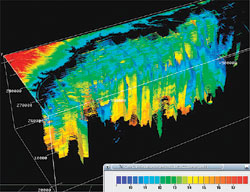Fig. 12. Pore pressure (ppg) predicted from trend-kriged inverted checkshots and sonic logs for deepwater wells released by MMS, for all locations where pore pressure exceeds 10 ppg and predicted velocity error (Fig. 10) is less than ±1,200 ft/sec. (Scale for land elevation above sea level is not shown.)

REAL TIME UPDATING

The pre-drill pore pressure model aims to incorporate all new information acquired while drilling to reduce the uncertainty, not only at the current depth, but also ahead of the bit. To reduce uncertainty, drilling operations closely monitor the well conditions and update the model in real time. New measurements of formation pore pressure and logging-while-drilling sonic data give further information with which to calibrate the pre-drill model and constrain the various parameters. This process is illustrated in Figs. 13 and 14.

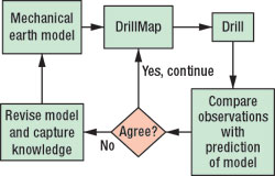Fig. 13. The procedure for updating the pore pressure prediction with data acquired while drilling.

Fig. 14. Implementation of the process for updating the pore pressure prediction with data acquired while drilling.

CONCLUSION

Knowledge of pore pressure is a key requirement for optimal development decisions in overpressured areas. Pre-drill pore pressure can be predicted using fit-for-purpose seismic velocities with a velocity to pore pressure transform calibrated to offset wells. The time required for such projects has been substantially reduced by building a pore pressure cube over the entire northern Gulf of Mexico, using data released by the Minerals Management Service (MMS).

All checkshots released by the MMS for the Gulf of Mexico were employed to estimate the 3D distribution of elastic wave velocity. The map of compaction coefficient k derived from this velocity model suggests that undercompaction, and associated risks from overpressure and/or shallow water flow, is likely to be largest in the vicinity of the continental shelf edge, particularly near the present mouth of the Mississippi. These results were obtained by assuming that velocity is a function only of vertical effective stress, defined as the difference between total vertical stress and pore pressure. Such regional knowledge of undercompaction trends should aid in the planning and safe drilling of future economic deepwater wells. 

LITERATURE CITED

1   Sayers, C.M., Woodward, M.J. and Bartman, R.C., “Seismic pore pressure prediction using reflection tomography and 4-C seismic data,” The Leading Edge, pp. 188 – 192, February 2002.

2   Doyen, P.M., Malinverno, A., Prioul, R., Hooyman, P., Noeth, S., den Boer, L., Psaila, D., Sayers, C.M. and Smit, T.J.H., “Seismic pore pressure prediction with uncertainty using a probabilistic mechanical earth model,” 73rd SEG Annual Meeting, Extended Abstracts, 2003.

3   Sayers, C.M., Smit, T.J.H., van Eden, C., Wervelman, R., Bachmann, B., Fitts, T., Bingham, J., McLachlan, K., Hooyman, P., Noeth, S. and Mandhiri, D., “Use of reflection tomography to predict pore pressure in overpressured reservoir sands,” 73rd SEG Annual Meeting, Extended Abstracts, 2003.

4   Sayers, C.M., Johnson, G.M. and Denyer, G., “Predrill pore pressure prediction using seismic data” Geophysics, pp. 1286 – 1292 Vol. 67, 2002.

5   Lizarralde, D. and Swift, S., “Smooth inversion of VSP traveltime data,” Geophysics, Vol. 64, pp. 659 – 661, 1999.

6   Traugott, M., “Pore/fracture pressure determinations in deepwater: World Oil, Deepwater Technology Special Supplement,” pp. 68 – 70, August 1997.

7   Hottman, C.E. and Johnson, R.K., “Estimation of formation pressures from log-derived shale properties,” Journal of Petroleum Technology, Vol. 17, pp. 717 – 722, 1965

8   Bowers, G.L., “Pore pressure estimation from velocity data: Accounting for pore pressure mechanisms besides undercompaction,” SPE Drilling and Completion, Vol. 10, pp. 89 – 95, 1995.