DRILLING / COMPLETION TECHNOLOGY

One-day gas well testing

Part 1 – In new wells with low permeability, a new, modified isochronal test method can give key information without extended well flow

Haldon J. Smith, Oil / Gas Consultant, Columbus, New Mexico, in association with Geo-Consultants, Ltd., Palma de Mallorca, Spain

resented here, for the first time, are methods, procedures and theory which detail how to deal with – in a quantitative and economic way – the analysis of transient gas flow behavior during a well test. Further, it is shown just how to do this in such a way that an operator developing a gas field need spend no more than a single day in testing any one well, regardless of how low the permeability or transmissibility (millidarcy feet per centipoise) of the test zone may be.

The thrust of this technology is thus focused on the most difficult zones to test, i.e., "tight" zones which do not stabilize readily. The special problems they present are solved. The author considers this to be a "ground breaking" presentation in that new analyses and relationships are presented for the first time.

The method noted above is presented in two parts. Part 1, described herein, introduces the subject with a background of conventional gas well testing limitations, particularly with formations that do not stabilize during a reasonable test period, and why a better procedure is needed. Basic features and limitations of the two types of backpressure tests now in existence – flow-after-flow and isochronal – are overviewed. And the new, modified isochronal test method adaptable to transient flow analysis is introduced.

Part 2 will continue the modified isochronal test introduction with an analytical procedure, including the Forchheimer equation shown in Part 1, and how it is used. Theory relating to pseudo-steady-state and transient flow is then presented. Finally, a generalized test program is developed to achieve desired objectives, involving a "decision point" by the test engineer.

Background / Introduction

There is no great mystery to the testing of gas wells if permeability of the producing formation is sufficiently high to allow stabilization of flowrate and flowing bottomhole pressure (BHP) within a reasonable time. Three rules of thumb from the author’s experience help tie down terms otherwise too relative:

1. Stabilization of flowrate: Rock-solid, or a variation of no more than ±5% measurement-to-measurement from the mean value, using 30-min. measurements.
2. Stabilization of flowing BHP: Rock-solid, or a variation of ±3% on a continuous measurement from the mean value; surface pressure readout desired for real-time monitoring.
3. Reasonable time: Anything up to, but not exceeding, 3 hr from opening.

The mystery does come, however, when a newly opened zone is found to have a low, or very low, permeability, such that it will not stabilize – in terms of flowrate or flowing BHP, or both – within a period of 3 hr or less from opening. In some cases, rate / pressure stabilization may require many hours, days or even weeks. Such extreme stabilization times are usually not economic, especially in offshore wells where testing is normally done with the rig still on location.

Three types of flow behavior. It is apropos to note that – within the author’s experience – gas wells, if they flow to surface, act in one of three ways upon opening:

1. Flowrate and flowing pressures stabilize quickly and remain consistent throughout the test period.
2. Flowrate / pressures fluctuate up and down within a usually narrow range throughout the test, reflecting a reverberation, or a sort of "echo" within the reservoir, perhaps from the hydraulic shock of sudden (especially surface) opening.
3. Flowrate / pressures decline noticeably and continuously throughout the dynamic test period, refusing to stabilize or even reverberate. If allowed to continue, this decline – depending primarily on reservoir system transmissibility – may continue for days or even weeks, or possibly until flow finally dies out.

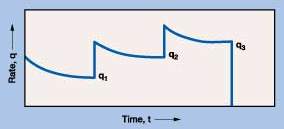
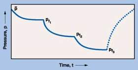
The first case above represents what reservoir engineers characterize as "pseudo-steady-state" flow. The second may resolve itself into pseudo-steady-state flow, or it may represent the early stages of long-term decline – extended flow will define it, if allowed.

The third case is the primary target of this article, since conventional testing wisdom dictates flow stability for valid test results. But such is not available in this case. Transient flow must be dealt with here – and in a quantitative manner.

New method for short-term tests. Now, finally, a method has been developed which allows the test to be performed in 24 hr or less, regardless of how low the test-zone permeability may be, or how useful / usable the data obtained therefrom is.

This article, in Parts 1 and 2, leads up to and explains the new method, after briefly reviewing pertinent points and caveats of background material. Then, a generalized optional test procedure is developed, that is open to the flexibility of real-time modification to adjust to real-time test data, such that all necessary test / reservoir data may be obtained from the test results in no longer than a 24-hr period, even with permeabilities less than one millidarcy.

This procedure may save operators many days of extra rigtime, if a zone happens to be exceptionally "tight," and may often allow stimulation to improve productivity at no great extra overall cost. The method may then be re-applied to re-evaluate the same zone after stimulation – and at the cost of only one additional rig day. Thus, a well may be completed and made a producer, which might otherwise have been abandoned.

Some discussion of the relationships of constants, or coefficients, between the Rawlins-Schellhardt and Forchheimer equations will be presented, without great mathematical detail. The approach is essentially practical in nature, but with sufficient theoretical overtones to provide adequate background to what is presented.

Backpressure tests, choke sequencing. Backpressure tests of gas well deliverability are multi-rate tests involving three or more flow periods on fixed chokes with flowrates, flowing pressures, etc., recorded as functions of time, usually at 30-min. intervals, exactly to the second. In the U.S., these tests are usually required by state law as a basis for allowables and for prorating purposes. Outside the U.S., they are usually not required, but are valuable for reservoir and production engineering studies, such as: evaluating the need for possible stimulation; sizing of flow and trunk lines; and comparisons of well performance and field development.

In gas well testing, two basic types of backpressure tests exist for determining and comparing deliverability: flow-after-flow and isochronal.

Each is discussed only briefly below, by way of review, as both are now well known and too much detail here would only be redundant. However, certain subtle caveats do apply, which may be overlooked by the less-than-diligent test engineer – these are highlighted.

First, a few words on choke sequence and test iron are in order. A well should always be opened on the smaller choke first. This reduces flowrate / pressure stabilization time to a minimum by introducing the smallest available dynamic change to the static reservoir equilibrium. It also avoids the otherwise unavoidable necessity for introducing a directionally-reversed dynamic change to that already established on the previous choke flow – a definitely undesirable action.

Next, in any flowing situation where it becomes necessary to change chokes directly from one to another without shutting in the well, a dual-flow, test-choke head with 2-in., direct-through bypass must be employed. The 2-in. bypass is also useful for initial cleanup, as will be seen later. No shut-in between chokes means exactly that; the test flowstream must not be interrupted even for a few seconds, if avoidable, when changing chokes. This applies exclusively to flow-after-flow tests.

Flow-After-Flow Tests

A flow-after-flow test comprises a series of increasing flow tests, on increasing choke sizes, beginning with an initial shut-in condition; ideally at initial static reservoir pressure, with no shut-in periods between choke changes. Graphically, it will look like the curves in Figs. 1 and 2.

This test was designed for wells which stabilize rather quickly, i.e., in less than about 3 hr from opening. Note in Fig. 1 that flowrate is steady near the end of each flow period. Note also, in Fig. 2, that flowing BHP is steady toward the end of each flow period, i.e., on each choke, flow reaches pseudo-steady state before change to the next-larger choke.

Fig. 1. Flow-after-flow test, rate vs. time.

Fig. 2. Flow-after-flow test, pressure vs. time.

This type of flow occurs only in reservoirs of relatively high permeability, thus, short stabilization time. No particular numerical criterion applies here, but reservoirs of one Darcy permeability, or more, will probably exhibit this flow pattern. It is also a function of reservoir thickness and overall size (drainage radius available) and gas viscosity.

In the above, since pseudo-steady state flow is achieved, the Rawlins-Schellhardt equation is best used for analysis:

Where:

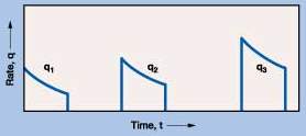
This conventional analysis is done graphically, plotting the difference of the squares of the pressures vertically, vs. the various corresponding flowrates horizontally. Usually, plots are made on a log-log basis only, to accommodate the magnitude of numbers involved. The result is a straight line, one point of data for each choke flow, and whose slope is l/n (vertical over horizontal). For multiple pseudo-steady-state flows, n is constant. Once n is determined, the performance coefficient, C, can be calculated from Equation 1, and the performance equation for that particular zone is complete.

Using the performance equation, absolute open-flow (AOF) potential is then calculated simply by setting pf equal to atmospheric pressure. This is the theoretical rate the well would flow if the formation face were somehow opened directly to atmosphere. It can never be achieved in practice, of course, because of wellbore geometry. It is used practically to compare one well’s performance to that of another well, and in setting allowables.

This figure, AOF, can and should be checked graphically on the plot before being reported. A common allowable is 20% of AOF. The multi-flow period is followed by a pressure buildup, for at least the same time as total flowtime, to ascertain permeability and any formation damage, skin, etc.

The above procedure was presented by Rawlins and Schellhardt in their landmark 1936, U.S. Bureau of Mines paper, and is still used today. However, it can best be used only if a well stabilizes quickly and achieves pseudo-steady-state flow during test-flow periods.

Isochronal Tests

Not all wells stabilize quickly enough to achieve pseudo-steady-state flows on test. For those which do not, the Rawlins-Schellhardt method noted above should not be used. However, the isochronal (equal time) test procedure was later designed for use in such wells. This test measures the transient deliverability of a well in a lower-transmissibility reservoir.

Correct application requires that each and every flow period begins from an originally-static reservoir condition. Therefore, intermediate shut-in periods must be of sufficient duration for pressure buildups to reach original static reservoir pressure at gauge depth.

In low- or very-low-transmissibility gas reservoirs, it may require days, or even weeks, for intermediate pressure buildups to reach original static reservoir pressure, even after relatively short flow periods. Thus, the isochronal gas well test does not, in itself, really solve the problem of extended test time – inevitably the result of inherently low transmissibility. But it is a way to deal with transient flow – though not always the best way available.

Pure theory, in an isotropic reservoir system, would have pressure buildups reflecting a mirror image of pressure drawdowns, except for one thing: during the flow period, reservoir fluid is removed to surface from the reservoir. Thus, the system which is building up is different than the system which drew down, by virtue of the mass and volume removed. This may be significant or not, depending on reservoir size / geometry.

Also, in practice, it is the author’s experience that nearly all hydrocarbon reservoirs are naturally fractured, to some degree. Fractures mean a non-isotropic system. And fractures themselves always have a higher permeability than unfractured blocks of the same reservoir. In such a situation, pressure drawdowns are primarily imposed on the high-permeability fracture system, but ensuing pressure buildups involve the whole network of fractures and unfractured blocks as well. Due to transmissibility variations and shifting emphasis, this inevitably brings into play a time difference.

For these reasons, drawdown and buildup times are usually unequal, and so their curves are not usually mirror images of each other. Graphically, the isochronal test looks like the curves in Figs. 3 and 4.

In Fig. 3, note that all flow times are equal, but pressure buildup times grow increasingly longer between them. Also, larger chokes produce larger transient flowrates, but they remain transient; that is, they do not stabilize before shut-in.

Fig. 3. Isochronal test, rate vs. time.

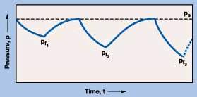
Fig. 4 shows how flowing and shut-in BHPs behave; flowing pressures also do not stabilize before shut-in. However, note that each pressure buildup does reach original reservoir pressure before the next opening; it is emphasized that this must occur as shown to validate the isochronal test procedure, regardless of how long it may take. The caveat is – this is the weakness of the isochronal test procedure.

Fig. 4. Isochronal test, pressure vs. time.

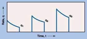
Finally, pressure buildup curves recorded on isochronal shut-ins require special treatment to be analyzed for permeability, because they were not preceded by stabilized, or pseudo-steady-state flow. Even so, the result will be somewhat in error.

In summary, the isochronal test procedure does provide a way to handle transient flow of gas wells, but it fails to solve the problem of required extended test time brought into play by the inherently low transmissibility of some reservoirs.

Modified Isochronal Tests

In view of the shortcomings of both test methods described above, a way was sought to deal effectively and quantitatively with transient flow, while at the same time limiting total testing to economically-acceptable and reasonable periods of time. Thus, the modified isochronal test procedure was introduced.

This procedure does not achieve (nor require) pressure buildup to original static reservoir values during shut-in periods. It is normally run with flow and shut-in periods all equal in length. As a result, this method will entail some error caused by unstabilized shut-in periods. This, however, is at least partially mitigated by the dynamics of the transient-flow analytical method used.

Its great advantage, from a practical viewpoint, is that however low the transmissibility of a reservoir may be, total test time required to effectively evaluate the gas zone can be fixed and limited beforehand. Graphically, the modified isochronal test procedure looks like the curves in Figs. 5 and 6.

In Fig. 5, note – first of all – that flow and shut-in times are all of equal length. Note also that production rates are transient, i.e., still decreasing at shut-in. And, of course, successively larger chokes create larger flowrates.

Fig. 5. Modified isochronal test, rate vs. time.

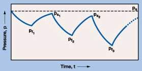
In Fig. 6, the most important point to note is that pressure buildups, limited as they are by fixed times, do not reach original static reservoir values. Next, note that flowing BHPs do not stabilize before shut-in; again evidence of transient-flow conditions caused by low transmissibility.

Fig. 6. Modified isochronal test, pressure vs. time.

A final pressure buildup can be taken to analyze for permeability but, again, will require special treatment and entail some error, however small. The special treatment consists merely of using an adjusted flow time to calculate the dimensionless time points for a Horner plot. Adjusted flow time is the total amount of gas recovered on test divided by the "average" of prior flowrate(s). While not scientifically accurate, because of the very nature of the test, the result will be the best approximation available under the circumstances.

One must always remember that the test analyst is dealing, in reservoir terms, not with a phenomenon of machine-like precision like a gear train or a clockwork, but rather with a randomly-varying geological system which has many unknown – and unknowable – variations, and almost certainly could not be described in precise mathematical terms even if they were known. Therefore, calculations in such a system can be, at best, macro-descriptive but certainly not mathematically precise. One cannot, and should not, expect too much from macro-mathematics applied to such a system. Still, it must be dealt with.

In transient-flow analysis of a modified isochronal test using 30-min. readings of flowrate and flowing BHP corresponding to each other, several readings are taken of each, for every flow period. Analysis of these data is best carried out by use of the Forchheimer equation:

Where:

Part 2 will analytically examine the above form of the Forchheimer equation and how it is applied, before proceeding with the other discussions noted earlier.

The author

Haldon J. Smith holds a professional PE degree from Colorado School of Mines (1953), a master of PE degree from the University of Tulsa (1956), and an MBA diploma from Alexander Hamilton Institute, of New York University. He worked 6-1/2 years in Venezuela for Creole Petroleum, followed by several years in France, Libya, Indonesia, Saudi Arabia, etc. – in all, more than 50 countries – mainly on reservoir studies / well testing. He has tested about 600 oil / gas wells, analyzed some 2,000 such tests and performed about 125 reservoir studies. He has been a full-time consultant since 1980, and has served 66 clients. His most recent significant work was 2-1/2 years in Bulgaria; he continues to be active.