Geologically consistent inversion results reduce uncertainty

Individual geophysical methods respond differently to particular earth properties. The most effective way to reduce risk when defining hydrocarbon resource is to integrate these data to construct the most complete earth model possible. This integration is challenging, because each method has different vertical and lateral resolutions, and each one has a wide range of possible models or “solutions” that will fit the field data. Another challenge is integrating a wide variety of data with different types of coverage. These include: 1) sparse, but high, vertical resolution well data; 2) sparse field geology observations; 3) 2D seismic or multi-physics lines; and 4) dense and/or continuous 3D seismic coverage.

MULTI-PHYSICS INITIATIVE

The industry is seeking to optimize the integration of multi-physics data to improve the accuracy and resolution of earth models. CGG launched a multi-physics imaging group to address these challenges. The integration process starts with the joint inversion of different datasets. Rather than using the different data types independently or in an interpretation sequence, the core work process will incorporate a larger sampling of different datasets for the depth inversion that will render the earth model.

By inverting controlled source electromagnetic (CSEM) jointly with seismic structural information, or airborne EM with geological outcrop dip/lithology, the group can produce a more reliable earth model using all the available information. This system helps interpreters, especially when they are on a tight timeline for drilling decisions. The joint inversion approach also helps geophysicists with the scale, resolution and distribution differences between the various datasets.

METHODOLOGY

A subsurface volume that can be interpreted reliably in terms of geologically relevant attributes is a desirable objective for products from depth inversion workflows. Geophysical data are inherently inaccurate, (noise, aliasing), and the inverse problem is commonly non-unique, so an implementation of constraint is required to recover reasonable output models.

Two cross-gradient inversion examples are provided, one where surface geological information is included in the input dataset, building on previously published work^1,2,3, and another integrating seismic data. The basic application covers the usual structural similarity objective, comparing the gradient fields of property volumes derived from different geophysical domains. A distinct advantage comes when gradient control from surface or subsurface geology, or any ancillary property set, is included during single or joint domain inversions of geophysical data.

Gallardo and Meju introduced the cross-gradient concept for the joint inversion of different geophysical methods.⁴ The idea was to quantify structural similarity between two property distributions, rather than inter-property correlation, by looking at the norm of the cross-product of their gradients. This norm is zero, if the directions of change in the two models are aligned. It is irrelevant, if the values of the model parameters increase or decrease in that direction. Likewise, the strength of the change does not matter. We add the cross-gradient term as an additional regularization term to the inversion cost function:

The cross-gradient concept maintains that two different datasets collected over the same geology should detect the same geological boundaries, albeit in different ways. Gradients of geophysical properties are an efficient way of understanding where the property, and thus the geology, is changing. Often one dataset might only show a very subtle gradient response over a geological boundary, but the cross-gradient method will still detect that boundary, if it finds a coincident response in the second dataset. Practically, cross-gradients are used as a regularization term in the inversion of the geophysical data.

The vectors m_A and m_B contain two different properties sampled on the same model grid. For a simultaneous joint inversion of two geophysical datasets, m_A and m_B are both part of the total model vector m; i.e. m_A contains resistivities while m_B contains the densities, and m is composed by concatenating them.² The additional regularization term comes with its own trade-off parameter γ. Using the cross-gradient part as sole regularization does not stabilize the inverse process adequately, so additional regularization, in the form of the smoothness term is required. We found it useful to keep γ constant, while adjusting β, in order to reach the desired misfit.

Instead of comparing the model gradients of two different property volumes inverted simultaneously, it is possible to introduce a priori gradients derived from an auxiliary model or dataset. In this case m_A is identical to the inverted model vector m, while m_B is the auxiliary a priori model that remains unaltered during the inversion. Since only the direction of change matters, arbitrary numerical values can be used to create an auxiliary model resembling geological structures. Alternatively, gradients can be defined directly without setting up a model containing nominal values, so instead of creating an auxiliary model m_B, the gradients m_B are used as inversion input.

The equation assumes that all model vectors contain dimensionless quantities. The overall magnitude of m_A or m_B is not relevant for the cross-gradient regularization, as it will only affect the strength of the regularization, which is adjusted by the trade-off parameter γ. It is possible, however, to scale the a priori gradients, based on how reliable the a priori information is in a certain part of the model, relative to other parts. For example, in the case illustrated below, where surface dips are used to regularize the inversion, the dip-derived gradients are scaled down with depth, to reflect that while the dips are well understood at surface, they are less so at depth.

STEERING WITH SURFACE GEOLOGY

Time-domain airborne EM data (CGG Helitem) were acquired by the service provider in the Alberta, Canada, foothills area, as part of a near-surface characterization program. The stand-alone (i.e. without cross-gradient) 2D and 3D smooth model inversions capture the main geological units, but the shapes of the anomalies fade out quickly, and dips are not obvious. Stand-alone smooth inversions generally identify the rough location of anomalous geology, but struggle to define the edges and shape of the causative body. By incorporating geological dips into the inversion using cross-gradient regularization, the structure of the main geological units is better defined.

Fig. 1. Map a) Surface geology with strike and dip points (blue ellipses); Map b) Interpolations of the input vectorial dip data onto a regular grid; Map c) SW-NE cross-section.

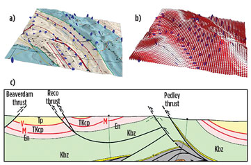
Ground measurements of dip and strike are available from a 1:50000 geologic map⁵ published by Langenberg and LeDrew, Fig. 1a. The accompanying interpreted cross-section, albeit adjacent to the AEM survey area, illustrates the compressive structural style, with outcropping steep thrusts cutting the related fold structures. The actual ground dip measurements were projected into data-poor areas along the mapped geological contacts. The surface dip data were interpolated component-wise between the ground dip measurements, with a minimum curvature spline in tension, as depicted in Fig. 1b. Gradient values were then mapped to the 3D reference model, starting from the first earth block downwards. While the dips are well-defined at the surface, they change with depth, to fade out the cross-gradient regularization. Accordingly, the gradients are increasingly smoothed downwards.

Integrating various datasets. When compared to the blind inversion results (Fig. 2a), both close to the surface and below, the steered inversion provides a more realistic structural model, Figs. 2b and 2c. In similar workflows, the code facilitates surface geology constraint of a range of single or multiple geophysical domain inversions, including potential fields and seismic.

Fig. 2. A slice from a 3D inversion of AEM survey data with: a) unconstrained inversion; b) surface-geology steered inversion; and c) close up on a different slice in the volume.

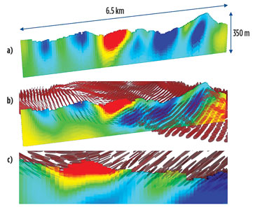
Red discs are co-rendered with resistivity to show the effect of the directional constraint on the orientation of the recovered structures. The consistency with the surface measurements is ensured through a high weight in the cross-gradient term in the shallow cells, faded to zero at increasing depth.

The steered inversion results in an image that is more geologically realistic. Consequently, these results are more easily interpreted, as they naturally define the edges of geo-bodies that can be used as inputs into other parts of the interpretation or inversion workflow. In this case, the resistivity inversion can be used to constrain seismic tomography in the near-surface.

STEERING WITH SEISMIC

In an offshore exploration application, the model steering uses depth-migrated seismic to constrain a controlled-source EM inversion. The main issue when integrating seismic and non-seismic data is the significant difference in resolution. Seismic images can be sampled at more than one order of magnitude higher than the meshes used for EM modelling. To bring the directional information from the seismic data to a resolution appropriate for EM, we employed the structure tensor.⁵ This operation is based on an eigenvalue decomposition of averaged gradients within a volume of interest, resulting in a vector field that captures the directions with the most significant variations.

Fig. 3. Seismic image-guided inversion of marine CSEM data: a) unconstrained inversion; b) image-guided inversion; c) detail of gradients derived from seismic image; d) gradients across EM cell boundaries are estimated with a structure tensor operator, to bring directional information from high-resolution seismic data to a scale appropriate for EM modeling.

For each cell of the EM inversion mesh, gradients from the seismic image are summed to construct the structure tensor matrix. The 2D formulation (easily generalized to 3D) is as follows:

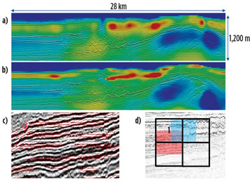
The eigenvectors of this matrix represent the directions of the main variation, whereas the eigenvalues represent the strength of the gradient. We incorporate this information in the auxiliary model, which is used for steering the EM inversion by means of cross-gradients. The example in Figure 3 is an application of this technique to marine CSEM data in the Norwegian Sea, whose inversion has been steered, based on a seismic image. The focusing of the resistive structures is enhanced, and the consistency with the seismic data is improved.

REDUCING RISK/UNCERTAINTIES

The quantitative use of surface or subsurface geological data during 2D and 3D inversion modeling provides a result that is consistent with all available data, which increases plausibility. This is accomplished through steering the inversion, using cross-gradient regularization, where the reference gradient model is derived directly from surface geology, conceptual structural models, or seismic volumes. The methodology is generic, and therefore expandable to derive a controlling gradient field from the range of subsurface attribute data available in exploration, development and production projects.

Various input datasets can be used to generate a reference gradient model for cross-gradient regularization. These can be sparse geological data, or high-resolution geophysical models that are related, due to their sampling of the same geological space. Furthermore, cross-gradients provide a way of including a range of both surface and subsurface data as inversion constraints. The result is an inversion that is consistent with all the available data, and usually of higher fidelity than stand-alone,  data-driven inversions.

This workflow is enhancing the adoption of a multi-geophysical data approach in exploration, development and production projects. Projects underway include near-surface characterization, using high-end airborne EM systems Resolve and Helitem, in the Permian basin, the Middle East and the Canadian foothills. A full-spectrum, broadband, airborne gravity gradiometry is also being similarly integrated to define drilling hazards like karsts, and for mapping salt and basin structures.  

ACKNOWLEDGEMENTS

The authors would like to thank CGG for providing the AEM data sets and facilitating the publication of this work.

REFERENCES

1. Scholl, C., S. Hallinan, F. Miorelli and M. D. Watts, “Geological consistency from inversions of geophysical data,” 79th EAGE Conference and Exhibition, Paris, France, June 12-15, 2017.
2. Scholl, C., J. Neumann, and M. D. Watts, “Geosteered 3D inversion of AEM data in rugged terrain,” 1st European Airborne EM Workshop, Turin, Italy, 2015.
3. Scholl, C., J. Neumann, M. D. Watts, S. E. Hallinan and S. Mulè, “Geologically constrained 2D and 3D airborne EM inversion through cross-gradient regularization and multi-grid efficiency,” Extended Abstracts ASEG-PESA, 2016.
4. Gallardo, L. A., and M. A. Meju, “Characterization of heterogeneous near-surface materials by joint 2D inversion of dc resistivity and seismic data,” Geophys. Res. Lett., 30, 1658, 2003.
5. Langenberg, C. W., and l. LeDrew, Geological Map: Coal Valley, NTS Mapsheet 83F/2, 1:50,000 map with cross-sections. Alberta Geological Survey Map 237, 2001.
6. Zhou, J., A. Revil, M. Karaoulis, D. Hale, J. Doetsch, S. Cuttler, “Image-guided inversion of electrical resistivity data,” Geophys J Int. 197 (1), 292-309, 2014.