Method proves itself for field monitoring of asphaltene treatment programs

Asphaltene deposition can result in significant costs and losses. Image: Baker Hughes.

Asphaltene deposition is a serious concern for operators, particularly in deepwater subsea systems, due to the immense capital costs of these developments; expense and challenges in performing remediation operations; and the potential for staggering amounts of lost or deferred production.^1,2 Consequently, it is imperative that asphaltene concerns are evaluated thoroughly for new deepwater subsea systems, prior to field development. If deposition concerns exist, effective asphaltene management programs must be developed and maintained.

Onshore, the situation is much different, because costs for drilling and completing wells, and for performing remediation operations, are dramatically lower. However, significant costs and losses for dealing with asphaltene deposition can still exist. Furthermore, in certain applications, such as CO₂ flood operations, the occurence of asphaltene deposition is almost assured. Thus, effective asphaltene management programs are also important onshore.

Asphaltene management programs can focus on prevention and/or remediation. For deepwater subsea operations, prevention is the primary focus. Remediation is very expensive, both in terms of cost and deferred production incurred. Onshore, production rates are generally much lower, and remediation is easier and less costly. Thus, in some cases, remediation may be an acceptable or preferred option onshore for asphaltene management. However, if effective economical methods exist, prevention will be favored.

The most common prevention method is to apply chemical asphaltene inhibitors. These inhibitors can help stabilize asphaltenes in crude oil, and, in some applications, reduce deposition significantly. The industry needs, however, to improve assessment of inhibitor application effectiveness. This includes predicting performance for new applications and in assessing performance during field application. Unfortunately, there is an inability in some fields to make good performance assessments, while products are being applied.

The Analytical Centrifuge Stability Analysis for Asphaltenes (ACSAA) method³ was developed as a simple, dead-oil, asphaltene stability method to help assess inhibitor performance. Although the method can detect fine differences in inhibitors’ ability to alter asphaltene stability, it is not a direct, live-fluid, high-pressure asphaltene deposition test. Consequently, on its own, the method only provides guidance on potential relative performance differences between inhibitors.

It is possible that correlations for field performance expectations could be developed by relating ACSAA testing to field data or high-pressure deposition data. Similarly, developing correlations for field expectations potentially could be accomplished from field monitoring measurements. In this instance, direct field performance results are related to the method. In the process, potential adjustments in the treatment program might be discovered that improve operations.

Fig. 1. Schematic of the sample orientation in the analytical centrifuge.

The field monitoring program discussed in this article is the first ACSAA monitoring application. It was applied to a North American field with a CO₂ – Water Alternating Gas (WAG) flood operation. It is an ongoing, proactive collaborative effort with the operator, to improve the understanding of chemical treatment performance and well expectations. However, given the nature of WAG flood operations, different wells within the field have varied complexities, affecting asphaltene deposition and inhibitor effectiveness.

Accordingly, developing correlations for treatment expectations is not as straightforward as would be expected in other types of fields. Nonetheless, good results have been obtained in more than a year of field monitoring data analyses. Examples presented illustrate the method’s ability to detect changes in field treatment dosage rates and to compare treatment chemistries. Attempts to correlate results to field expectations also are discussed.

METHOD DESCRIPTION

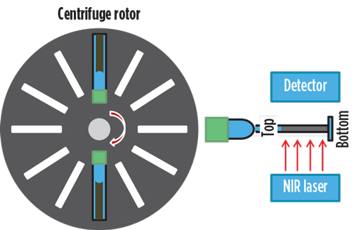
The ACSAA method uses an analytical centrifuge that spins samples while measuring the transmittance of near-infrared (NIR) light shone through the entire sample length. A multi-position rotor enables simultaneous analysis of up to 12 samples. Figure 1 shows a schematic of the analytical centrifuge.

Fig. 2. Sedimentation in an unstable dispersion, evaluated with an analytical centrifuge.

Analytical centrifuges evaluate dispersion stability. By monitoring changes in light transmission along an entire length of a sample during centrifugation, changes in the dispersion’s solid concentration, at various levels of the sample, can be detected. As the dispersed solids scatter light, transmission of light increases in areas losing solids and decreases in areas gaining solids. As a result, sedimentation or creaming can be observed in a quantitative manner.

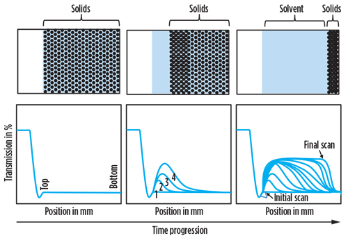
Figure 2 shows sedimentation in an unstable dispersion, observed using an analytical centrifuge. As the dispersion breaks down, solids separate from the carrier solvent and move toward the bottom of the centrifuge vial. As separation continues, light transmission increases in the sample’s top portions. The transmission increase progresses down the length of the sample, as solids settling continues. Thus, at the bottom of the sample, the transmission can decrease, due to increased solids settling.

For the analytical centrifuge used in this work, the instrument’s software utilizes transmittance data to calculate a normalized potential for solids flocculation and settling. This calculation parameter is termed the instability index. This index is a calculation of the change in integral transmission between time 0 and time t, normalized by the maximum theoretical transmission, resulting in a calculated value from 0 to 1. An instability index of 0 indicates a sample is completely stable, with no change in the transmittance trace occurring. Conversely, the larger the instability index, the more unstable is the sample.

Similarly, in this method’s testing, asphaltene stability is gauged by monitoring the change in transmittance, as the sample is centrifuged during the test. The behavior is similar to solids settling in a dispersion, when a destabilizing solvent is added to the petroleum sample being evaluated. As the asphaltenes destabilize and separate from petroleum fluids, transmittance increases, because asphaltenes are the species in petroleum that strongly absorb light. Consequently, the change in transmittance is used to monitor asphaltene stability by determining relative changes in asphaltene content in the different regions, or entire length, of the centrifuge sample. If asphaltenes are destabilized, the transmittance trace behaves similarly to Fig. 2, and the destabilized asphaltenes will largely settle to the bottom of the centrifuge vial. The instability index is then used as a relative indicator of asphaltene stability.

DETAILS OF FIELD MONITORING

Field details. The field discussed is a North American CO₂ – WAG operation, with hundreds of producing wells. Naturally flowing wells, and wells on ESPs or rod pumps, are present. Production rates vary dramatically within the field, from less than 1 bopd to ~325 bopd. Water cuts range from ~70% to 95%. Similarly, the CO₂ content varies dramatically in the different wells, depending on location and stage of the WAG operation. Percentages of CO₂ vary from ~10% to 85%. The crude oil is medium-gravity with an average asphaltene content around 3 wt. %. However, asphaltene contents from samples taken in the monitoring program from various wells have varied from ~1 to 6 wt. %.

The field experiences periodic, various well/equipment failures. Rod pump failures are from hung-up rods/pumps. ESP failures are caused generally by plugged tubing or plugged pump intake/stages that lead to broken shafts or overheated motors. Failures in flowing wells are caused by plugged well tubing, wellheads or flowlines. Most plugging is from asphaltene deposition, but scale and formation fines can also cause, or contribute to, plugging.

Correspondingly, most wells are treated with asphaltene and scale inhibitor to mitigate fouling problems. When applied, inhibitor injection is either through capillary strings or annular injection. The latter is more prevalent in the field, because capillary strings are not available and/or economical to install in many wells.

Field complexities affecting assessments. Because this is a WAG operation, complexities (which vary over the WAG cycles) exist that affect asphaltene stability and deposition, as well as an inhibitor’s effectiveness. In particular, asphaltene stability depends highly on the amount of CO₂ that is mixed into the crude. If enough CO₂ mixes in, asphaltenes will be destabilized. Lower amounts can shift asphaltene phase-stability boundaries, such that asphaltenes are destabilized during production, as pressure drops occur.

The location where CO₂ mixing and destabilization occur also affects the types of problems that result. If destabilization and deposition occur deep within the reservoir, it should not cause production problems. However, if it occurs in the near-wellbore region or in the production tubing, it is a serious concern. Near-wellbore formation damage can reduce productivity dramatically. Similarly, deposition within the well can hurt production by restricting or plugging well tubulars and/or causing ESP or rod pump failures.

The location where CO₂ mixing and destabilization occur also determines the effectiveness of inhibitor treatments. Ideally, the inhibitor should be added to the crude oil prior to asphaltene destabilization. If added afterwards, the inhibitor will be less effective or might not provide any inhibition. For all the applications discussed, the inhibitor was injected into the well via capillary or annular injection. Consequently, if destabilization occurs beforehand in the reservoir, the inhibitor might perform poorly, even it is actually an effective chemistry. This is one of the complexities and challenges present in evaluating treatment performance in this and other CO₂ flood fields. The actual, changing flow dynamics of the flooding during the WAG cycles are not completely known. 

In addition, other factors contribute to pump failures, such as scale deposition and electrical equipment malfunctions. Although the failure cause is usually determined when the pumps are pulled, the non-asphaltene failures can interfere with developing valid run life statistics.

Another issue for any field monitoring program is obtaining representative samples. An unknown factor, prior to starting field monitoring, was how much sample variation would occur. Would the samples truly represent production occurring during the period that they were acquired?

Wells selected for monitoring. Field monitoring was started with five wells (two untreated and three treated with asphaltene inhibitor). Four additional wells (two untreated and two treated) were added later. However, one of these treated wells was dropped from monitoring.

This article focuses on the results obtained from the remaining eight trial wells over approximately one year. Some other wells were subsequently added to the monitoring program, but with less-frequent sampling. The large number of wells in the field, and the effort involved to collect and analyze samples, precluded inclusion of every well in the program.

Sampling frequencies for the eight wells ranged from approximately three to nine samples/month. Inhibitor A was used in each of the treated wells. Inhibitor A was switched in two of the four treated wells later to trial the performance of an alternative, Inhibitor B, and, concurrently, to determine the field monitoring method’s ability to detect potential performance changes.

Sample collection and processing. Production return samples were collected in 240-ml prescription bottles from the wells for analysis. The samples contained varying amounts of crude and produced water; often emulsified. The samples were heated in a water bath at 80°C, for at least 7 hr, to break emulsion. The heating was sufficient in breaking the emulsion, except, in some cases, small amounts of emulsion pad still existed near the oil-water interface. After heating, the prescription bottles were set aside for later testing.

For the instability index measurements, 80-µL pipette sub-samples were taken directly from the top level of the crude in the bottles for most of the analyses. If only small amounts of crude oil (less than 15 ml) were present in the bottle, sub-sampling directly from the bottle was problematic, due to the thin oil layer. In these cases, it was difficult to ensure the pipette sub-sample would not also extract water or emulsion pad material so these samples were handled differently.

The production return samples discussed here were collected between July 2014 and August 2015. Data presented in figures from the different wells are plotted as a function of days from the start of the field monitoring program. July 1 was defined as Day 1 of the program, although the actual first samples were taken on July 3.

RESULTS OF FIELD MONITORING

In previous asphaltene inhibitor testing, the ACSAA method has proven to have good precision. Experimental variability is generally better than ± 5 %. In tests using the same oil sample, the method has reproducibly detected changes in asphaltene stability, resulting from small changes in inhibitor dosage rates or in inhibitor chemistry.³ Consequently, the method should detect changes when field inhibitor treatment rates or products are changed. However, in a WAG field, changes in the oil from production returns can occur, depending on the cycle stage or life of the WAG operation. Uncertainty exists in whether the oil pushed from the reservoir to the well will be the same consistently.

Fig. 3. Instability Indices for samples from untreated wells #1 and #2.

In addition, how the crude oil interacts with CO₂ and water can make a difference. For example, are asphaltenes precipitated from the crude? How much? Does this precipitation occur prior to, during, and/or after inhibitor injection? Alternatively, are non-representative samples with higher amounts of interfacially active/asphaltene species obtained, due to the specific samples taken being primarily water with small amounts of associated crude oil? Additionally, in some wells, the inhibitor applications were down the annulus, so there were some questions about how steady or continuous was the inhibitor delivery rate. As a result, depending on when the exact sample was taken, could it potentially have a higher or lower dose rate than the average delivery rate? The availability of samples from untreated wells and performing additional analyses (like simply measuring asphaltene contents), was important in answering some of the variability questions.

Fig. 4. Instability Indices for samples from untreated wells #3 and #4.

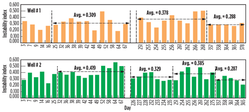
Untreated well results: Determining typical variations. Instability indices are shown in Fig. 3 for samples taken from the first two untreated wells in the field monitoring program. Shown are analyses from samples taken during different sampling periods over more than a year. There are some variations in having occasional spikes or dips in data from samples taken days apart and in variations of averages taken over different sample periods. The variations are not so great that it would interfere with evaluating asphaltene inhibitor influence, particularly if multiple samples are taken over a range of dates and evaluated.

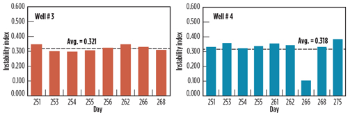
In contrast, in the other two untreated wells, very consistent crude oil characteristics were obtained, over relatively short time periods. Figure 4 shows instability indices for the other two untreated wells (#3 and #4) for samples taken over a month-long time period between March and April 2015. Note, with the exception of two analyses, the instability indices are all within 5% of the average instability index for the respective wells. Nevertheless, the presence of periodic outliers demonstrates that drawing conclusions, based on analyzing multiple samples, is highly recommended.

Fig. 5. Instability Indices for samples from treated wells #5 through #8.

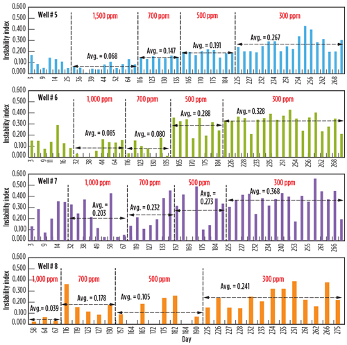
Treated well results: Detecting changes in product dose rates. For the treated wells, asphaltene inhibitor treatment rates were decreased progressively, from an initial 1,500 ppm or 1,000 ppm, to 300 ppm, to determine the sensitivity in detecting dose rate changes in the production return samples. Figure 5 shows the instability indices for the four treated well samples, as the inhibitor dose rates were lowered. Although there are some spikes and dips with some individual samples, in each case, the average instability index over the different sample periods shows a consistent trend of increasing instability with decreasing dosage. Consequently, the data show that the method is suited to monitoring changes in the production return samples. However, again an average over a range of samples should be reviewed.

Determining treatment thresholds and correlating well run life expectations. In addition to optimizing treatments, either through adjusting dose rates or applying new chemistries, a goal for this field monitoring application was to provide information to assist in determining treatment levels required to prevent or extend pump failures to acceptable run lives. This goal requires developing correlations on various product treatment rates on well/equipment run lives. What follows is a quick, simplified example on how to do this.

Fig. 6. Comparison between untreated wells and wells treated with 500 ppm Inhibitor A.

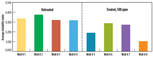
Figure 6 compares the averaged instability indices of the untreated well versus treated well samples at 500 ppm. As expected, untreated wells have higher instability indices. Generally, untreated wells are not treated because asphaltene deposition is less severe, and the wells’ run lives are sufficiently long enough that it is more economical not to treat. It could be surmised that these wells’ asphaltene stability levels are sufficient to yield acceptable run lives. And, perhaps, treating other wells to achieve at least the same stability (~0.3 instability index) would provide satisfactory inhibition and well run life times.

Figure 5 shows that instability indices are below 0.3 in Wells #5 and #8 when treating at 300 ppm with Inhibitor A. Hence, if a treatment threshold were set to achieve an instability index of 0.3, 300 ppm would be an acceptable treatment rate for these wells. For Wells #6 and #7, however, instability index averages are above 0.3 when treating at 300 ppm, but lower at 500 ppm with Inhibitor A. Therefore, in applying the same criteria, the optimal treatment rate would be between 300 ppm and 500 ppm.

Setting a treatment threshold, based on assumptions discussed from Fig. 6 data is, of course, not a rigorous means to best define treatment requirements. As discussed earlier, not all wells are the same with respect to CO₂ breakthrough, flow dynamics, and other potential contributing factors to deposition. Ideally, individual guidelines would be determined for each well. However, the above example illustrates simply, how data could be used to aid optimizing treatment rates.

Individual well guidelines could, potentially, be determined over the course of a few failure cycles. However, it is not desirable to wait and allow failures. Instead, developing a continual running field database with information on production, failures, and chemical treatment history is needed over all the field wells to provide data to help make treatment decisions. Over time, as more information is obtained, better  treatment decisions will be made.

Fig. 7. Comparison of Instability Indices before, and after, switching asphaltene inhibitors.

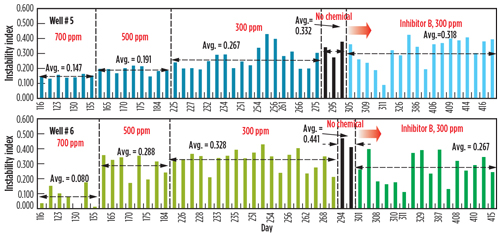
Comparing different inhibitor products. To improve treatment effectiveness and cost efficiency, a different asphaltene inhibitor (Inhibitor B) was suggested for field trial. The recommendation was based on laboratory testing of untreated field crude oil samples (although not from the exact wells trialed), with the alternative inhibitor showing better performance. Thus, the alternative inhibitor was trialed on wells #5 and #6. Figure 7 compares production return analyses from the two wells before, and after, switching products. In between switching products, inhibitor treatment was halted for three to four days, to collect untreated baseline data.

As seen in Fig. 7, over the first one-and-a-half weeks, the instability indices appeared to decline when using Inhibitor B in both wells. Longer term, the difference between the two inhibitors was less apparent. For Well #6, Inhibitor B’s performance at the 300-ppm treatment rate appeared to be slightly better. Approximately 20% and 40% reductions in the instability indices were obtained over Inhibitor A and untreated averaged data, respectively. For Well #5, the overall production results with Inhibitor B were slightly worse than those with Inhibitor A. The average instability index was higher than Inhibitor A data and almost equivalent to the untreated data. It is uncertain why better results were not obtained. In analyzing fluid compositions, there did not appear to be changes in crude characteristics that could skew performance comparisons shown in Fig. 7. Because other inhibitor options were planned for future trials, further efforts were not pursued to more closely evaluate performance differences between Inhibitors A and B.

CONCLUSIONS

Examples from more than a year of field monitoring analyses for a North American CO₂-WAG flood operation were presented to show the ACSAA method’s ability to detect changes in field treatment dosage rates and compare treatment chemistries. The results illustrate the method’s potential for use in monitoring and improving asphaltene treatment programs. For the field discussed, continued field monitoring and collaboration with the operator is ongoing. 

ACKNOWLEDGMENT

This article is based on OTC paper 27129-MS, which was presented at the Offshore Technology Conference in Houston, Texas, May 2–5, 2016.

REFERENCES

1. Creek, J., “Freedom of action in state of asphaltenes: Escape from conventional wisdom,” Energy and Fuels, vol.19, p.1212-1224, 2005.
2. Kurup, A. S.; J. Buckley, J. Wang, H. Subramani, J. L. Creek and W. G. Chapman, “Asphaltene deposition tool: Field case application protocol,” OTC paper 23347, presented at the Offshore Technology Conference, Houston, Texas, April 30–May 3, 2012.
3. Nagarajan, N. R., M. Stratton, P. Juyal, A. Yen and J. Nighswander, “Asphaltene issues and challenges in the Gulf of Mexico: Current technology gaps and path forward,” presented at the 14th International Conference on Petroleum Phase Behavior and Fouling, Rueil-Malmaison, France, June 10-13, 2013. 
4. Jennings, D. W., R. Cable and G. Leonard, “New dead-crude oil asphaltene inhibitor test method,” OTC paper 25113, presented at the Offshore Technology Conference, Houston, Texas, May 5-8, 2014.
5. Jennings, D. W., R. Cable and M. Newberry, “Asphaltene stability analyses for optimizing field treatment programs,” SPE paper 170677, presented at the SPE Annual Technical Conference and Exhibition, Amsterdam, The Netherlands, Oct. 27–29, 2014.