Do data mining methods work? A Wolfcamp shale case study

The study’s objective was to compare the relative utility of several statistical and machine learning methods to predict production quality. Photo courtesy of Baker Hughes.

Data mining for production optimization in unconventional reservoirs brings together data from multiple sources, with varying levels of aggregation, detail and quality. Tens of variables are typically included in data sets to be analyzed. There are many statistical and machine learning techniques that can be used to analyze the data and summarize the results.

These methods were developed to work extremely well in certain scenarios, but can be terrible choices in others. The question for both the analyst and the consumer of data mining analyses is, “What difference does the method make in the final interpreted result of an analysis?”

This study’s objective was to compare and review the relative utility of several univariate and multivariate statistical and machine learning methods in predicting the production quality of Permian basin, Wolfcamp shale wells. The data set for the study was restricted to wells completed in, and producing from, the Wolfcamp. Data categories used in the study included the well location and assorted metrics capturing various aspects of the well architecture, well completion, stimulation and production. All of this information was publicly available. Data variables were scrutinized and corrected for inconsistent units and were sanity-checked for out-of-bounds and other “bad data” problems.

After the quality control effort was completed, the test data set was distributed among the statistical team for application of an agreed-upon set of statistical and machine learning methods. Methods included standard univariate and multivariate linear regression, as well as advanced machine learning techniques, such as Support Vector Machine, Random Forests and Boosted Regression Trees.

Fig. 1. The graphic shows the gross structure of the Delaware basin and Central basin platform features of the Permian basin of West Texas. Study wells are bubble-mapped.

The strengths, limitations, implementation, and study results of each of the methods tested are discussed and compared to those of the other methods. Consistent with other data mining studies, univariate linear methods are shown to be much less robust than multivariate non-linear methods, which tend to produce more reliable results. The practical importance is that when tens to hundreds of millions of dollars are at stake in the development of shale reservoirs, operators should have the confidence that their decisions are statistically sound. The work presented here shows that methods do matter, and useful insights can be derived regarding complex geosystem behavior by geoscientists, engineers and statisticians working together.

BACKGROUND

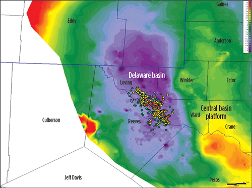
The study area is within the Delaware basin of West Texas. The area encompasses parts of Loving, Ward, Winkler and Reeves counties, Texas. Figure 1 is color-contoured on the top of the Wolfcamp and highlights the basin structure in the greater area. The deep basin is shown in purple, and the shallowest Wolfcamp contours are in red. Well locations are bubble-mapped on top of the contours. The bubble map color scheme shows the best monthly oil production per completed foot of lateral (log10 scale), shown in red, with the poorest wells shown in purple. Wells are selected mainly from Phantom field and are listed in the public data as being Wolfcamp (451WFMP) completions.

Wolfcamp, in the study area, comprises a thick section of unconventional reservoir, and publicly reported, vertical well log tops indicate a gross interval ranging in thickness from 2,000 ft to 4,000 ft. It is subdivided generally into zones A-D. Our data set contains 476 Wolfcamp shale horizontal wells with production histories from the Permian basin. Three production metrics serve as target variables in each method, including the cumulative oil production of the first 12 producing months in bbl (M12CO), the maximum monthly oil production of the first 12 producing months in bbl (MMO12), and production efficiency derived by dividing MMO12 over total lateral length in bbl/ft (MMO2CLAT).

Fig. 2. Histograms of selected predictor variables.

As predictor variables, we pulled over a dozen assorted metrics covering various aspects of the wells: geographic location, well architecture, well completion and stimulation. We know that reservoir quality is crucial to well production. However, it depends on permeability, porosity, viscosity and other metrics, which are not practically available for large number of wells in any current data base. Instead, we used X-Y surface locations (SurfX/SurfY) as proxies of reservoir quality in our work. Well architecture variables included operator (opt2), well azimuth (AZM), drift angle (DA), true vertical depth in ft (TVDSS), and cumulative lateral length in ft (LATLEN). The operators have been made anonymous and categorized from A to F. All operators with less than 20 wells were grouped into one class. AZM and DA were taken from the actual directional survey in the well’s completed lateral section. LATLEN was calculated as the difference between the measured depth (MD) of base perf/sleeve and that of top perf/sleeve.

Fig. 3. Histograms of selected predictor variables.

Well completion variables included completion year (COMPYR) and number of completion stages per well (STAGE). Well stimulation treatment data were derived from IHS data by aggregating stage-by-stage entries, including total proppant amount in lb (PROP), total fracture fluid volume in gal (FLUID) and average proppant concentration as the ratio of the previous two (PROPCON). We scrutinized these variables and ran a data cleansing job, based on their distribution and the empirical experience of a subject-matter expert. For example, a PROPCON value of 30 lb/gal is erroneous since the theoretical threshold is 25 lb/gal and most practical values are less than 10. It is also worthy of mention that not every well in our study has reported values for all variables. It is common to have missing values in real-world datasets, especially those from public resources. The analytical methods being compared here have different tolerances and mechanisms for handling missing values.

EXPLORATORY DATA ANALYSIS

Fig. 4. Scatterplot matrix of selected predictor variables.

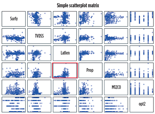
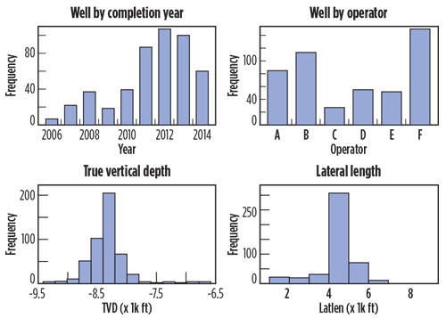
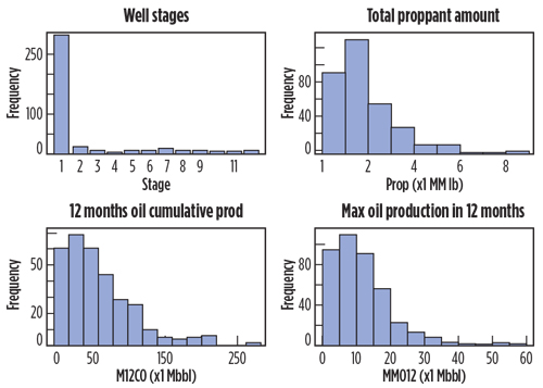
The histogram is probably the most widely used univariate apparatus for visualizing continuous variables (barplot for categorical variables). We used it to review the characteristics and distribution of each variable. From Figs. 2 and 3, we can easily see that the wells were completed between 2006 and 2014, with most completed in the last four years. LATLEN centered around 4,000-5,000 ft, with a range from 1,000 ft to more than 8,000 ft. Both PROP and M12CO were skewed heavily to the right, as well as MMO12. The scatterplot matrix in Fig. 4 can be used to identify pairwise trends among variables and unusual data points, such as leverage points and outliers. We can see a clear increasing trend between PROP and LATLEN from the highlighted cell, as well as between M12CO and LATLEN. Neither trend is close to linear. The production metric, M12CO, didn’t depend solely on any variable, and we need to conduct a multivariate analysis to reveal the complex relationship.

METHODS AND IMPLEMENTATIONS

To evaluate and compare the performance of the different methods, we adopted two objective metrics, average absolute error (AAE) and mean squared error (MSE). AAE is defined as the expected value of the absolute “error”, E|y- ŷ|, which is the difference between y, the observed production metric and ŷ, the fitted value coming out of a model. In practice, the AAE is estimated, using n pairs of responses y_i and predictions ŷ_i, as shown below.

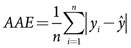
The definition of MSE is similar to AAE, and it measures the expected squared “error” E(y-ŷ)². The MSE is also estimated empirically, using the formula below.

Note that AAE has the same unit as the corresponding production metric y, but MSE is measured in squared units. In this analysis, the models were trained, using the full Wolfcamp dataset, and the AAE and MSE were computed by using predictions on that same dataset. As such, the results shown below describe the quality of the model fit on the data used to train the model. To properly evaluate the utility of these models on independent test data, a larger dataset may be required. Refer to the final section of the article for further discussion on this topic.

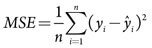
Ordinary least squares regression. The first method we applied was multiple linear regression, also known as ordinary least squares (OLS) regression. A linear relationship was fitted as:

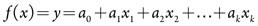
to minimize the difference between the observed and fitted values, where y is the target variable and x = [x₁, x₂, . . ., x_k] is the vector of values for the k predictor variables. The model’s simplicity comes with a set of strong assumptions. Also, the OLS model requires the completeness of the data, and all wells with missing variables were omitted during the fit. As an example, only 319 of the 476 wells had M12CO values, and we would delete another 148 wells in the OLS model due to missing values.

Fig. 5. Production observation vs. prediction from OLS model.

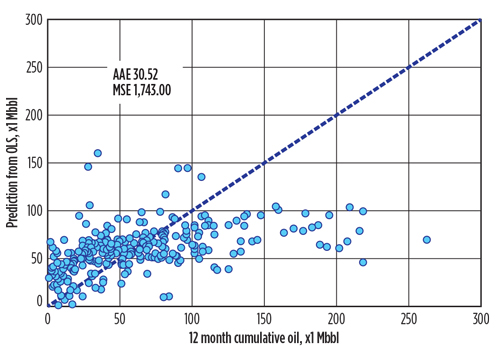
To compare with other methods fairly, we imputed the missing values, based on the similarity of the observations. Figure 5 shows the scatterplot between the reported M12CO and the fitted values from the OLS model, built upon the imputed data set. Theoretically, for a perfect model that fits every data point exactly, we should be able to see all points aligned on the diagonal dashed line. It provides a straightforward way to evaluate the goodness of fit. In our case, most points deviate from the line, which indicates that the OLS model did not fit the data well. The AAE was about 31 Mbbl for the cumulative oil production in the first 12 producing months, and the MSE was 1.743 MMbbl.² The average of reported M12CO was 60 Mbbl, and the median was 50 Mbbl.

There are several methods that can be used to improve model performance. One option is to perform a transformation of some of the predictor variables (e.g., log transformation), which may alleviate any violations of the normality assumption. Another option is to apply shrinkage methods (ridge regression and/or LASSO) to reduce the influence of multicollinearity, which was expected between PROP and FLUID, etc. However, we have limited space and will not discuss these remedy approaches in this article.

Support vector machines. Support vector regression (SVR) is a technique closely related to the use of support vector machines (SVMs), which are used widely in classification tasks. In the case of SVR,¹ the regression function has the form

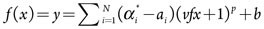
where v₁, v₂, . . ., v_N are N support vectors, and b, p, α_i α_i*, are the parameters of the model. The parameters are optimized with respect to ε-insensitive loss,² which considers any prediction within ε of the true value to be a perfect prediction (i.e., zero loss). During the parameter estimation, the support vectors are also selected from the training dataset. Since the model is only specified through the dot product v_i^t of the support vectors and the predictors, the “kernel trick” can also be used. This replaces the dot product v_i^t with a kernel function K(v_i,x), which can produce highly non-linear regression fits.

Fig. 6. Production observation vs. prediction from SVM model.

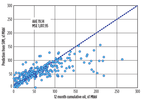
The SVR model was fit, using the radial basis kernel K(v_i,x) = exp (-γ|vi –x|²). Like the OLS model, the missing values were also imputed before fitting the model. The results in Fig. 6 show a modest improvement over the OLS regression result. The AAE drops from 31 Mbbl to approximately 19 Mbbl, and the MSE drops from 1.743 MMbbl to 1.018 MMbbl.²

Random forests (RF)³ are ensemble machine learning methods that are constructed by generating a large collection of uncorrelated decision trees, based on random subsets of predictor variables and averaging them. Each decision tree can be treated as a flowchart-like predictive model to map the observed variables of subjects to conclusions about the target variable. Trees capture complex interaction structures in the data and have relatively low bias, if grown deep. The averaging step in the algorithm provides a remedy to reduce the variance, due to the noisy nature of trees. Unlike standard trees, where each node is split at the best choice among all predictor variables, each node in a random forest is split, at best, among a subset of predictor variables chosen randomly at that node.

Fig. 7. Production observation vs. prediction from RF model.

For those wells with incomplete predictors, random forest imputes the missing values, using proximity. The proximity is a measure of similarity of different data points to one another in the form of a symmetric matrix, with 1 on the diagonal and values between 0 and 1 off the diagonal. The imputed value is the average of the non-missing observations, weighted by the corresponding proximities. Other that the imputation, the setup of random forest is quite user-friendly and only involves two parameters: the number of predictor variables in the random subset at each node and the total number of trees. Random forests and the gradient boosting method in the next section are both decision tree-based. Their predictor variables can be any type, numerical or categorical, continuous or discrete. They automatically include interaction among predictor variables in the model, due to the hierarchical structure of trees. They are also insensitive to skewed distributions, outliers and missing values. These properties enable them as “off-the-shelf” methods, which can be applied directly to the data without a lot of time spent on data preprocessing and parameter tuning.

Fig. 8. Relative importance of the predictor variables from RF.

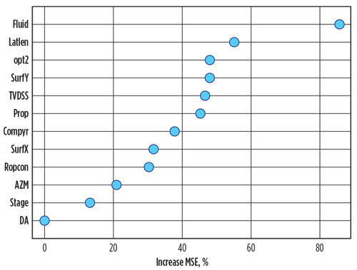
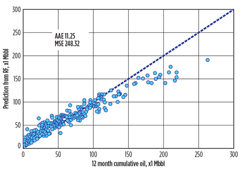
Figure 7 shows the scatterplot of the reported M12CO and the predicted values from the random forest model, with four features in each split and 5,000 trees. The data points were much closer to the diagonal dash line than those in the OLS model, which indicated that the random forest model had a better fit. The numeric evaluation also confirmed that AAE was about 11 Mbbl, and the MSE was 248 bbl.² Both were much smaller, compared to previous results. The random forest model also produced the two additional pieces of information shown in Figs. 8 and 9. Figure 8 contains the ranked, relative importance of the predictor variables. The relative importance measures the prediction strength of each variable by calculating the increase of MSE, when that variable is permuted while all others are left unchanged. The rationale behind the permutation step is that if the predictor variable was not important to the production, rearranging the values of this variable will not change the prediction accuracy by much. The top six drivers of M12CO were FLUID, LATLEN, opt2, SurfY, TVDSS and PROP.

Fig. 9. Partial dependence plots of the top six drivers from RF model.

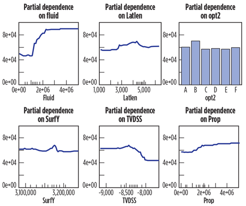
The partial dependence plots in Fig. 9 show the marginal effect of each individual variable on the prediction of the top six drivers. In each plot, the effect of all other variables was integrated out by averaging over the trees. The ticks on the x-axis of each plot are deciles of the predictor variable. According to these plots, those wells with 2.5 MM gal of fracturing fluid, around 4,500 ft of lateral length, from operator B, Y surface location of 3.17 MM units, TVD beyond 8,500 ft and more than 3 MM lb of proppant were more likely to have better cumulative production in the first 12 producing months. Wells with different FLUID values could have as much as more than 40 Mbbl difference in production. The fracturing job size, including PROP and FLUID, had a positive impact on the production. However, when it reached a certain level (2.5 MM gal for FLUID and 3 MM lb for PROP), the effect was marginal.

Gradient boosting model. The idea of boosting is to gain prediction power from a large collection of simple models (decision trees) instead of building a single complex model. The trees in a gradient boosting model (GBM)^4,5 are constructed consequentially in a stage-wise fashion, as compared to being constructed in parallel, in a random forest model. Each tree is introduced to compensate the residuals, or shortcomings of the previous tree, where the shortcomings are identified by negative gradients of a squared error loss function.

Fig. 10. Production observation vs. prediction from GBM model.

The final model can be considered as a linear regression model, with thousands of terms, where each term is a tree. The missing value issue is handled in GBMs with the construction of surrogate splits. The key step in a tree model is to choose which predictor (and where) to split on at each node. We use non-missing observations to identify the primary split, including the predictor and the optimal split point, and then form a list of surrogate splits, which tries to mimic the split of data by the primary split. Surrogate splits are stored with the nodes and serve as a backup plan in the event of missing data.

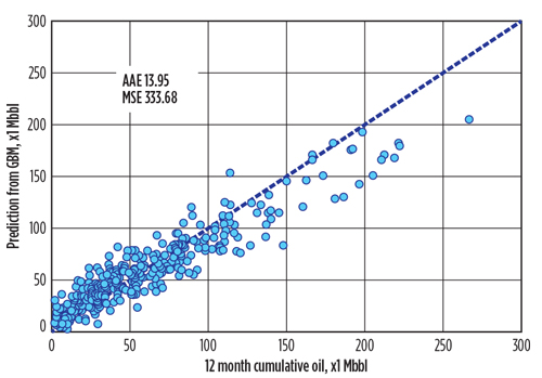
If the primary splitting predictor was missing in modeling or prediction, the surrogate splits will be used in order. An example is that we may use PROP or LATLEN to mimic the split of data in the absence of primary split of FLUID. The surrogate split utilizes the correlation between predictor variables to mitigate the negative impact of missing values. Figure 10 shows the scatterplot of reported M12CO and the predicted values from a GBM with a learning rate of 0.005, tree complexity of 5 and bag fraction of 0.5. The performance of the model is similar to that of RF with AAE at about 14 Mbbl and MSE at 334 Mbbl.²

Fig. 11. Relative influence of the predictor variables from GBM model.

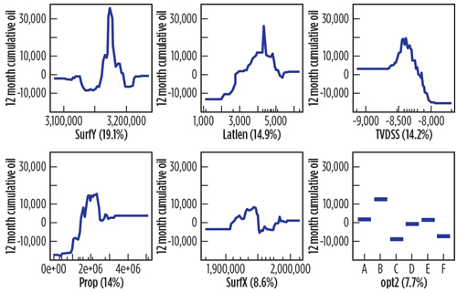
The gradient boosting model also produces a relative importance plot and partial dependence plots like the random forest does. The relative importance here is defined differently from that in random forest. It is based on the number of times that a predictor variable was selected for splitting, weighted by the squared improvement to the model as a result of each split, and averaged over all trees. The relative influence in Fig. 11 was rescaled with a total sum of 100. The top six drivers were SurfY, LATLEN, TVDSS, PROP, SurfX and opt2. The partial dependence plots in Fig. 12 indicated that those wells—with Y surface location of 3.17 MM units, 4,500-ft lateral length, true vertical depth near 8,400 ft, 2 MM lb of proppant, and from operator B—were more likely to have higher production. The predictions along the y-axes have been centered by subtracting their mean due to program setting. Wells with different SurfY locations could have more than 30 Mbbl difference in the production and wells from operator B were expected to have 20 Mbbl more production than those from operators F and C.

DISCUSSION & CONCLUSIONS

Fig. 12. Partial dependence plots of the top six drivers from GBM model.

We implemented several methods on the Wolfcamp data set, including OLS, SVM, RF and GBM. These methods have different tolerances for missing values, one of the most common issues in real world data sets. OLS and SVM simply omit the data points with missing values. RF imputes missing values, based on the proximity of the data points, and GBM creates surrogate splits as a workaround in the event of missing data. The two tree-based methods are more resistant to the missing values. In terms of overall fit on the full data measured by AAE and MSE, RF performed best among these methods, followed closely by GBM. SVM showed moderate improvement over OLS, which served as a benchmark model in our study, Table 1.

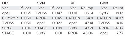
In each model, the predictor variables have different levels of contribution in predicting the target variable. To evaluate the variable importance in OLS and SVM, and compare the ranking with those from RF and GBM, we adopted a metric based on the R2 measure of goodness of fit. Each variable was systematically removed from OLS and SVM models, one-by-one. The R2 of the reduced model was then compared with that of the full model, and the difference of R2, or, the R2 loss, served as a measure of the importance of that variable. Table 2 shows the lists of the top six influential variables from all methods.

Table 1. AAE and MSE from the models.

TVDSS and opt2 appeared in each list. The geographic location (SurfX and/or SurfY) also had strong impact on the production in each model. The influence of the fracturing job size (FLUID and/or PROP) was recognized in all models except OLS. RF model ranked FLUID the most important predictor variable, with a large margin over others. GBM put more weights on the geographic location. According to the relative importance of the RF model, the top six drivers upon M12CO were FLUID, LATLEN, opt2, SurfY, TVDSS and PROP. The top six drivers from GBM model were SurfY, LATLEN, TVDSS, PROP, SurfX and opt2. The only different variable was FLUID replaced by SurfX in GBM.

Table 2. Variable importance from the models.

Despite the fact that these variables were ranked differently in two models, we can see that the marginal effect of each driver was captured similarly in these two models, after comparing the corresponding partial dependence plots. For example, wells with surface Y-location near 3.17 MM units are more likely to have higher production after accounting for the effects of the other predictors. Wells from operator B are more likely to have higher production than those from other operators.

Do data mining methods matter? The short answer is yes. According to the practice on the Wolfcamp dataset, tree-based methods, RF and GBM, required less pre-processing time on the raw data. They were also more resistant to common data quality issues and provided better predictions than others. The outputs of variable importance and the partial dependence plots helped to reveal key drivers and their nonlinear impact on the production. Therefore, they were preferred choices for similar plays.

Table 3. AAE and MSE for MMO12 from the models.

Besides the target variable M12CO, we also conducted parallel analysis on MMO12 and MMO2CLAT. Due to the similarity of the analysis, the details of the procedure were not described here. Tables 3 and 4 show the corresponding fits on MMO12 and MMO2CLAT, respectively. The model performance metrics in Table 1 were computed by comparing actual and predicted values on the same data used to train the models. To evaluate what the performance of the models might be on independent data sets, we tried to split the data set by holding out 20-30% of the data points as a test set. The models were built using the other 70-80% of the dataset. The performance metrics on the training set were similar to those from the full data models shown in Table 1. However, these models did not predict as well on the reserved test set, as they did on the training set, which points to an overfitting issue. A few approaches, including using less features in the models through variable selection and reducing the size of decision trees through pruning, have been carried out but did not show much improvement on the problem.

Table 4. AAE and MSE for MMO2CLAT from the models.

One factor making it difficult to do a full, robust analysis on model performance is the relatively small sample size in this dataset. There were 319 observations with non-missing response values, and only 171 observations with no missing predictor values. At such small sample sizes, performance results will be impacted heavily by which observations are selected randomly for the hold-out test set. With a larger dataset, we will be able to better evaluate these models, using a similar hold-out approach or a k-fold, cross-validation procedure. The Wolfcamp shale data set is only a simple example in our industry. There are also other machine learning methods, such as MARS, neural network and deep learning that have not been included in this comparison work. It would be interesting to run these models to extend our knowledge of their application on more oil and gas data sets. The analyses included in this article were conducted in R6, using the packages e1071⁷, random forest⁸, and GBM.^{9, 10} 

ACKNOWLEDGEMENTS

This article is based on SPE paper 173334, presented at the SPE Hydraulic Fracturing Technology Conference held in The Woodlands, Texas, Feb. 3-5, 2015. Parts of this work are based on, or may include, proprietary data licensed from IHS.

REFERENCES

1. Drucker, H., C. J. Burges, L. Kaufman, A. Smola and V. Vapnik, “Support vector regression machines,” Advances in Neural Information Processing Systems, Vol. 9, pp. 155–161, 1997.
2. Vapnik, V., The Nature of Statistical Learning Theory, New York: Springer, 2000.
3. Breiman, L., “Random forests,” Machine Learning, Vol. 45, No. 1, pp. 5–32, 2001.
4. Friedman, J., “Greedy function approximation: A gradient boosting machine,” Annals of Statistics, Vol. 29, No. 5, pp. 1189–1232, 2001.
5. Elith, J., J. R. Leathwick and T. Hastie, “A working guide to boosted regression trees,” Journal of Animal Ecology, Vol. 77, No. 4, pp. 802–813, 2008.
6. R Development Core Team, “R: A Language and Environment for Statistical Computing,” R Foundation for Statistical Computing, Vienna, Austria, 2014.
7. Dimitriadou, E., K. Hornik, F. Leisch, D. Meyer and A. Weingessel, “e1071: Misc Functions of Department of Statistics,” TU Wien. R package version 1.6.,” 2011.
8. Liaw, A. and M. Wiener, “Classification and Regression by randomForest,” R News, Vol. 2, No. 3, pp. 18–22, 2002.
9. Ridgeway, G., “Generalized boosted models: A guide to the gbm package,” 2007.
10. Ridgeway, G., “gbm: Generalized Boosted Regression Models. R package version 1.6-3.1.,” 2010.
11. Hastie, T., R. Tibshirani and J. Friedman, The Elements of Statistical Learning: Data Mining, Inference, and Prediction, New York: Springer, 2001.