Preprocessing of offshore platform-integrated marine monitoring system data: What to do with unusual values or trends?

Full-scale measurements provide indispensible information for validating the behavior of an offshore oil platform; however, they often contain some observations that deviate from a majority of other values.  

Igor Prislin, Soma Maroju and Kevin Delaney, BMT Scientific Marine Services

This article addresses the challenge posed by measurement data on offshore platforms that doesn’t fall into the norm. Specifically, it deals with measurements obtained by offshore platform-integrated marine monitoring systems—such as metocean data, GPS data and structural data—that, at a glance, have unusual values or trends. In each case, a solution for how to treat unusual values is presented. The article discusses some unusual episodes in full-scale measured data and suggests possible treatments for such unusual values. Proper treatments of the measured data can enable marine assurance engineers to make the right decisions and avoid possible damages to the system or even a shutdown of production due to faulty alerts.¹

INTRODUCTION

Measured data that contain unusual or unexpected values cannot be used directly in automatic data analyses, and results interpretation of the unexpected values could be erroneous for a variety of reasons. Detecting and understanding data errors and “rare” event syndromes are particularly important when statistical techniques are applied to the measurements. If data are used unconditionally, the calculated statistics may be biased. It is important to differentiate between errors in the data and unexpected values that are products of real, but rare, events. It is unquestionable that interpretation of rare events is a challenging task, particularly if no numerical simulation or model test results are available.

It is common practice to validate the most recent measured data by comparing it with the previously measured data under similar conditions. When previous measurements are few, or when simulated results are not available, unbiased techniques for detecting unusual values or trends in the data, such as Artificial Neural Networks (ANNs) and Kalman filters, are useful additions to common statistical trend analyses.

Unusual data need not always indicate a platform integrity failure. Rather, they may originate from instrumentation failures. For example, a sudden “jump” in the GPS data can indicate an instrumentation issue as simple as a change in satellite constellation or a change in atmospheric conditions. On the other hand, the “jump” can indicate a sudden drift of a platform due to breakage of a mooring line. The latter is a real event that indicates a serious platform integrity issue requiring immediate attention.  The ability to differentiate between the two is essential for deciding on a proper course of action.

MARINE INTEGRITY MONITORING

Marine integrity monitoring is a cluster of activities that includes data acquisition, processing and evaluation. Data acquisition, and related instrumentation systems, and data evaluation from the operational standpoint that have been discussed by other authors will not be repeated here.^1–6 This article concentrates on processing and evaluating measured data, after the data become available to analysts. Three major groups of data used for assessing marine integrity monitoring are discussed: environmental data (e.g., waves, wind and current), platform global motions and structural responses, particularly tendon tensions.

MEASURED DATA—MAIN OBJECTIVES

Measured data serve primarily to confirm that the platform behaves as designed under design conditions and to identify behaviors of the platform under unusual conditions to assess the platform’s safety and structural integrity.

It is particularly challenging to interpret unusual measured data that has not been considered during the design process but that may affect the safety and integrity of a platform. Although such data may represent “real” deviations from normal platform function, they also may be outliers, which do not affect the platform safety or structural integrity. Given drastically different implications of the two, it is essential that unusual data is properly categorized.

Visual aids—e.g., visual inspection of time series, or checking the distribution of data values by levels of a categorical variable (variance, skewness, kurtosis)—are the traditional methods of understanding the data. This procedure is always preferred and should be one of the first steps in data analysis, because it will quickly reveal the most obvious outliers or will point to valid results that require additional attention. However, visual inspection requires a knowledgeable and specially trained data analyst. In addition, visually inspecting a massive amount of data collected on an offshore platform, 24 hours a day, 7 days a week, represents an arduous and expensive task. Therefore, having an automatic process to identify and treat the outliers in a bulk of measured data is preferable. If this method uncovers some anomalies, then the most critical events can be additionally inspected and analyzed using visual tools.

ENVIRONMENTAL DATA

The two main environmental sources of data are waves and ocean currents.

Waves are usually measured from a platform by air-gap radars installed at the corners on the lowest deck around the platform. The number of air-gap sensors varies from platform to platform. These air-gap sensors are used to measure relative surface elevation with respect to the platform fixed point. As the sensors are moving with the platform, the actual surface elevation is calculated by subtracting the sensor motions from the measured air-gap values around the mean value. This procedure is simple in principle but requires accurate measurements of the air-gap sensor itself.

The undisturbed “zero” water level is not measured but is approximated with the mean level, which is calculated from the air-gap measurements. Measured air-gap data could be contaminated with outliers caused by physical reasons, including ocean spray formation around the sensor and a loss of a return signal due to reflections from obstacles between the sensor and the sea surface (boats, hanging hoses, etc.).

Outliers represent an observation that is significantly different from the rest of the data. Outliers affect not only the extreme values, but also the mean and higher statistical moments, making results invalid for any further analysis. Importantly, there is not an accepted precise definition of “significantly different,” and the criterion has to be carefully selected.

The simplest way to isolate outliers is by applying a univariate statistical test. The test detects one outlier at a time and expunges it from the data set. The process is iterated until no outlier is detected.

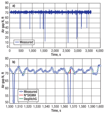
The test statistic is defined as a multiple of the ratio between the offset from the mean value and the standard deviation (known also as “3σ or 6σ edit rules”). This test is simple and robust only if there are just a few outliers in a large set of data and if the mean and standard deviations are known in advance and are not estimated from the same data set. Otherwise, outliers in the data set (Fig. 1a) significantly affect the calculated mean and standard deviation from the data and the test becomes biased and unreliable.

There are many additional statistical tests similar to the one described above. They include Chauvenet’s, Pierce’s and Grubbs’ tests, to mention a few.⁷ They are all based on the assumption that the measured data are normally distributed. More stable methods are based on unbiased statistics such as inter-quartile-range computation—for example, using the median rather than the estimated mean value and the Median Absolute Deviation (MAD) rather than the standard deviation.⁸ The MAD scale estimate is usually defined as S = 1.483 x median {x_i – x_median} so that the expected value of S is close to the standard deviation for the uncontaminated, normally distributed data.

Applying MAD estimates to the air-gap data, the outliers are identified and the values are replaced with  spline-type interpolated data, Fig. 1b. In practice, it is also common to replace an outlier with the “last good” value or with the median value, or to just skip the point, rather than to find an interpolant. Each procedure has its advantage and disadvantage depending on the objectives of the data analysis.

Fig. 1. Measured air gap with outliers (a) and after they have been removed and smoothed (b).

The MAD technique can be efficiently used to identify the outliers in other types of measured data, such as the riser tension data.

In spite of all their positive aspects, statistical techniques, such as MAD, should be applied with caution. If the measured data is nonstationary, the variation in the data may not necessarily be attributed to outliers. For example, observation of the wave power spectrum during the passage of a hurricane reveals that the wave spectra are in a transient state because the magnitude and period of the peak of the spectrum vary in time. In this case, the largest peak could be falsely interpreted as an outlier.

Ocean current near the free surface in the vicinity of an offshore platform is usually measured with a Horizontal Acoustic Doppler Current Profiler (HADCP). The HADCP is typically installed on the platform hull 50–100 ft below the free surface.

The current measurement is based on the Doppler shift between the frequencies of the transmitted acoustic pulse and the echoes received from different bins on the acoustic beam. Even though the instruments are already provided with the built-in capabilities to reduce noise and glitches in the recorded values, there are cases when recorded values may still contain outliers that require careful examination and treatment.

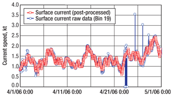
An example of the measured 10-min. average horizontal current speed near the surface is shown in Fig. 2. The figure shows the measured signal with some outliers and the post-processed results with the outliers removed. In this case, a method based on a coherence value calculated over all bin pairs is implemented, rather than the MAD method. The 10-min. average horizontal current speed should not vary significantly from one bin to another. Thus, the bins with a relatively high cross-coherence index (e.g., ≥ 0.8) are selected, and the measured current speeds are averaged over all these bins to estimate the actual current speed. The values for incoherent bins are rejected as outliers.

Fig. 2. Ten-minute average near-surface current speed measured with an HACDP.

This method has been tested on many occasions, and it seems to be a robust and reliable estimator for the horizontal current speed. The current direction is estimated as an average value using the same bins. Unfortunately, this method cannot be used to treat vertical current profile measurements. The profile is usually more sheared than uniform; thus, the speeds at different bins lack coherence.

PLATFORM GLOBAL MOTIONS

An estimate of platform global motions is not a simple task. It requires accurate and high-resolution measurements and careful data post-processing. Conventional methods for measuring six degrees of platform motions are based on measurements of accelerations, angular rates and linear displacements using (D)GPS technology. As measured linear accelerations are coupled with angular motions due to the effect of gravity, the gravity effects should be removed from accelerations before double integration.

In addition, linear displacements as double-integrated accelerations are not accurate enough at low frequencies—primarily for numerical reasons—and should be substituted with the direct (D)GPS displacement measurements at these frequencies. Numerical integration of a harmonic linear acceleration (e.g., sway acceleration) at frequency ω is simply a product of the acceleration and the integration operator G = ω-2. At very low frequencies, the operator G grows hyperbolically and, for a signal with a low signal-to-noise ratio, the integration of noise can be overamplified. This can significantly skew the platform displacement results, including basic statistics. Similarly, the platform angular dynamic motions are affected by artificial amplification of noise due to a single integration of angular rates. In the latter case, the integration operator is H = ω-1.

A simple remedy to the errors due to an unrealistic integration of noise would be to filter out all low-frequency components. However, simple filtering is not recommended because this method eliminates estimates of low-frequency platform motions, which are important for understanding mooring line and riser loads.

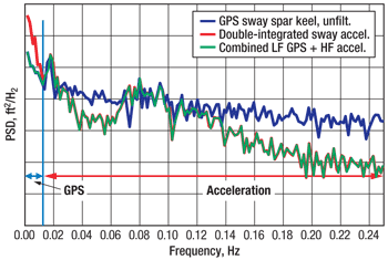
A solution is to combine displacement measurements from (D)GPS at very low frequencies and the double-integrated accelerations at higher frequencies. The merging frequency can be determined as the frequency at which the displacement calculated from acceleration starts to deviate significantly from the (D)GPS displacement, Fig. 3. This figure also reveals that the (D)GPS signal is noisier than double-integrated acceleration at higher frequencies; thus, the (D)GPS signal should not be used for displacement estimates at the high frequencies. The combined displacements are blended into a single signal in the frequency domain and then transformed back to a displacement time series by the inverse Fourier transform.

Fig. 3. Combination of sway GPS and acceleration measurements.

Another important issue in data processing is to decide on the start and end points of the post-processed time series if numerical filtering is involved. Due to the Gibbs phenomenon, the data at both ends of the filtered signal are overamplified. These artificial large values represent “numerical outliers” and should be eliminated from the results. There are at least three solutions to minimize this problem:

• Cut off the ends of the post-processed time series by a few percent of the total length after filtering
• Use a tapered rather than rectangular window (e.g., Hamming window).
• Extend the time series on both ends before filtering and then remove the extensions after filtering to match the length of the original time series. In this case, the total length of the time series is preserved.

Finally, the main purpose of measuring the platform global motions is to estimate the platform kinematics (accelerations and velocities) at non-measured locations. The calculation involves a combination of all motion-sensor data through rigid-body kinematic equations:

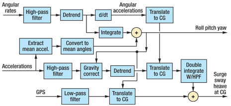
where ŕ_p, ω and ὠ and  are vectors defining the distance between points O’ and P, angular velocity and angular acceleration, respectively. The calculated kinematics depend on all six-degrees-of-freedom measurements, and an error in a single measured channel would influence all final results. For this reason, careful preprocessing of each measured motion channel is important. The flow chart shown in Fig. 4 represents the procedure for post-processing the platform motions.

Fig. 4. Flow chart for post-processing procedure for calculating platform motions.

A more advanced approach to this procedure would include a Kalman filter to reduce the motion artifacts from a noisy motion signal. After the six-degrees-of-freedom motion data are processed and translated at the platform, it is always a good practice to recalculate the platform accelerations and compare the results with the original, measured values. This procedure ensures that the post-processing algorithm is working correctly. It also reveals a degree of data smoothing and quality of interpolation for missing points or outliers.

STRUCTURAL MONITORING

A more advanced method in evaluating measured data is an Artificial Neural Network (ANN).The ability to learn and generalize by example is the principal characteristic of an ANN. ANN models can be used to forecast and identify a variety of hidden patterns in the real data from an offshore platform, including platform attitudes and riser integrity. They can also be used to detect faulty instruments without running expensive and complicated analytical models.⁹

With the expectation of developing deeper and larger oil production systems, the Tension Leg Platform (TLP) Tendon Tension Monitoring Systems (TTMSs) are usually designed for high resolution and high sampling rates in order to maximize information about the system responses to environmental loadings. This imposes additional requirements on the data acquisition system to make it functional in a variety of conditions, including major failures of the instruments. Thus, a dual-redundant load cell system can be used to acquire the tendon tension data. However, even with dual redundancy used in measuring the tensions, errors can creep in if care is not taken to validate the quality of the data.

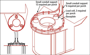
The TLP tendon tension and moments (Fig. 5) are measured using three dual-redundant strain gauge load cells per tendon, located 120° apart on top of a tendon. At least three load cells are necessary to calculate top bending moments on each tendon. At the same time, the tendon tension is estimated as an average of the three load cell signals. Dual redundancy of a TTMS is achieved by installing two strain gauge resistance bridges on each load cell, which, in an ideal situation, record the same loads. The average of these two bridge signals provides the estimated tension from a load cell. However, if one or both bridges becomes faulty, the estimated force per load cell will be wrong if the algorithm does not throw out the values from a faulty bridge. Hence, the identification of faulty bridges is essential to make correct estimates of the tendon tensions.

Fig. 5. Typical porch-based tendon tension load cell layout.        .

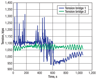
Usually, an algorithm based on a priori defined threshold values is implemented to identify faulty bridges. This deterministic approach is not flexible enough to capture a faulty signal (Fig. 6) when it is out of the predetermined range. In this case, an ANN model becomes extremely valuable as an unbiased and self-adjusting tool for detecting faulty bridge signals.

Fig. 6. Measured tendon loads with two bridges.

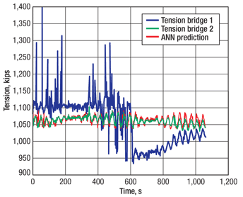
The main idea behind the ANN model is to train it over time when the TTMS is new and works as designed. The training of the ANN is based on a variety of measured input parameters, such as environmental loads, platform global motions, ballast and weight conditions. The dependent output variables are the bridge signals. After the ANN model is trained and validated, the measured bridge signals can be compared in real time with each other and with their ANN-predicted values. In Fig. 7, the results show that the tension signal from Bridge 1 is questionable and should be eliminated from further analysis. Proper detection and discrimination of faulty signals also reduces the number of false alarms.

Fig. 7. Measured and ANN-predicted tendon tensions.

CONCLUSIONS

Results show that automated methods for detection of outliers and unusual data are useful aids, particularly when a vast amount of measured data needs to be interpreted in real time. However, it is highly recommended that specific events of a particular interest still be carefully interpreted by a knowledgeable and well-trained data analyst who can prevent making the erroneous conclusions and improper actions that may happen in blind data processing.   

ACKNOWLEDGMENT

This article was based on OTC 19933 presented at the Offshore Technology Conference held in Houston, May 4–7, 2009.

LITERATURE CITED

 ¹ Prislin, I., Rainford,, R., Perryman, S. and R. Shilling, “Use of field monitored data for improvement of existing and future offshore facilities,” Paper D5 presented at the SNAME Maritime Technology Conference & Expo, Houston, Oct. 19–21, 2005,
²  Edwards, R. et al., “Review of 17 real-time, environment, response, and integrity monitoring systems on floating production platforms in the deep waters of the Gulf of Mexico,” OTC 17650 presented at the Offshore Technology Conference, Houston, May 1–4, 2005.
³  Prislin, I. and M. Goldhirsh, “Operational supports for offshore platforms—from system integrity monitoring to marine assurance and safety,” paper 57006 presented at the International Conference on Offshore Mechanics and Arctic Engineering, Estoril, Portugal, June, 15–20, 2008.
⁴  Goldsmith, B., Foyt, E. and M. Hariharan, “The role of offshore monitoring in an effective deepwater riser integrity management program,” OMAE 29479 presented at the Offshore Mechanics and Arctic Engineering Conference, San Diego, Calif., June 10–15, 2007.
⁵  Irani, M. B., Perryman, S. R., Geyer J. F. and J. T. von Aschwege, “Marine monitoring of Gulf of Mexico deepwater floating systems,” OTC 18626 presented at the Offshore Technology Conference, Houston, April 30–May 3, 2007.
⁶  Perryman, S., Chappell, J., Prislin, I. and Q. Xu, “Measurement, hind cast and prediction of Holstein Spar motions in extreme seas,” OTC 20230 presented at the Offshore Technology Conference, Houston, May 4–7, 2009.
⁷  Schenck, H., Theories of Engineering Experimentation, 3rd ed. Washington, Hemisphere Publ. Corp, 1978.
⁸  Huber, P. J., Robust Statistics, New York, Willey, 1981.
⁹   Prislin, I. and S. Maroju, “Development of artificial neural network models for offshore platform correlation study,” BMT Scientific Marine Services, Internal R&D Report, SMS-01-MGT-1664R-0001-01, 2007.