Interpretations from either data set alone may be incorrect.
K. René Mott, Seismic Micro-Technology Inc.; and Veronica Hunt, Fairfield Industries Inc.
Explorationists are constantly searching for data and tools to evaluate and reduce drilling risk. Drilling a non-producing well is generally costlier than evaluating all possible risk based on the available data before drilling. Hence, in the initial phase of the operation, gathering data to determine if the drilling target will prove worthwhile is critical.
This article presents a post-stack analysis of seismic data from a field with 15 producing wells in a standard federal lease in the Gulf of Mexico. The analysis includes the following attributes: amplitude, spectral decomposition, dip of maximum similarity and instantaneous Q, in addition to well log information. The objective is to provide an overview of best practices to determine the pay signature within the seismic dataset, reduce the inter-well stratigraphic interpretation risk, define anomalies by understanding their fundamental cause and reduce structural trapping risk.
OVERVIEW
The seismic data used in this article was acquired by Fairfield Industries using two parallel lines of receivers, with five shot lines taken between the two receiver lines. This type of swath acquisition provides the interpreter with superior data for analysis. All data was processed using Kirchhoff pre-stack time migration.
The field consists of 15 producing wells. The area is under production with many levels of pay in the field. The zone of interest, at 2.6 sec. in the seismic data, will be represented using both geological and geophysical data.
WELL TIE AND PAY SIGNATURE
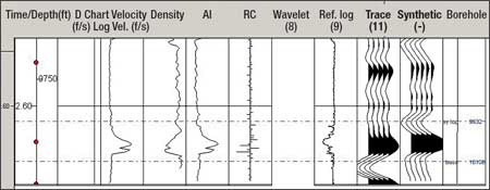
Using a forward model created from the sonic well log to create a synthetic seismogram, an explorationist can determine if the data is rotated from zero phase and how the top of the sand will express itself seismically, preferably as a peak-to-trough relationship, with the zero crossings about the trough representing the top and base of the reservoir zone.
The synthetic data also indicates a hydrocarbon pay signature for the data set, Fig. 1a. These logs-including time to depth, density and other logs that indicate the pay sand-are shown to the left of the two seismic traces. The left trace is actual seismic data, while the right is a synthetic computed from the sonic log. The signature is modeled to be a peak-trough-peak response. The peak-trough-peak signature is exactly what the seismic data exhibits at just below 2.6 sec. as delivered by the processing company, indicating that the area is worth exploiting for hydrocarbons.
|
|
|
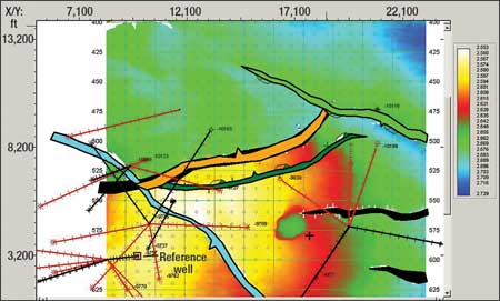
Fig. 1. a) The synthetic seismic is correlated to the survey data, showing the well tie and pay signature of peak-trough-peak. b) The resulting time-structure map from the time reflector tied from the synthetic data is shown.
|
|
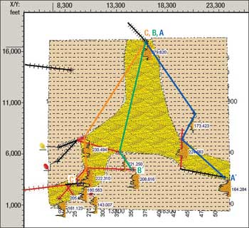
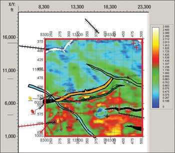
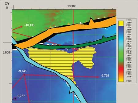
The map (Fig. 1b) shows faults that were interpreted from time amplitude and similarity data, the latter of which will be substantiated later. The faulting in the northern region is down to the basin and most likely syndepositional. The faulting in the southern portion of the block is counter-regional, down to the coast and antithetic to the regional depositional faults off screen to the north of the image.
The time-structure map illustrates the time-structure interpretation on the negative reflector tied from the aforementioned synthetic. The green to blue map colors illustrate the time structural lows, and the reds to whites demonstrate the time highs. The basic structure is a syncline trending northeast to southwest bounded on the south by a structure that is regionally higher to the west, centered on the circular green anomaly.
DEFINING THE STRATIGRAPHY
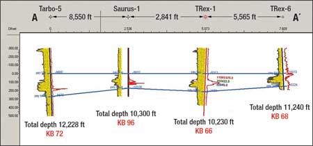
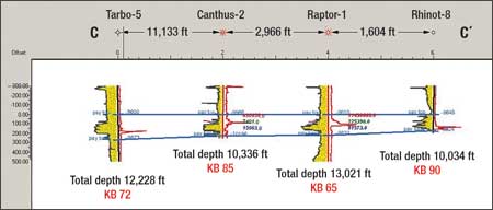
Figure 2a displays a stratigraphic cross-section along line A-A’ in the eastern portion of the block arranged so the top of the sand is a datum to help illustrate the deposition in the area at the 2.6-sec. interval. The northern well to the left shows a very thick overall interval from the top to the base of the zone-about 150 ft thick, thinning due east and then relatively thickening to the southeast. The yellow intervals are the net sand intervals within the overall zone.
|
|
|
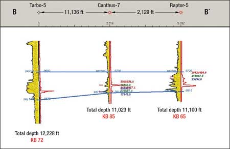
Fig. 2. a) A north-south-oriented stratigraphic cross-section on the eastern portion of the study area shows the thick sands to the north, thinning to the east and thickening again to the southeast. b) A second north-south-oriented stratigraphic cross-section in the center of the area shows the thick interval to the north, which thins to the south. c) The third stratigraphic cross-section on the western edge of the area illustrates the thinning of the sands to the southwest. d) A map of the combined data shows the facies and net sands resulting in a single feeder channel bifurcating into two lobes, east and west..
|
|
Figure 2b shows a structural cross-section along line B-B’ down the center of the area illustrating the thickest portion in the northern well and thinning to the south in this area. Figure 2c shows how the stratigraphy along line C-C’ is distributed in the western portion of the study area-thick to the north but relatively thinner to the southwest. Figure 2d is a map with combined postings of the isopach values for the zone of interest along with the log signature over the same interval. (Lines A-A’, B-B’ and C-C’ are shown on the map.) Log signatures are a portion of the well log over an interval, and the interval is defined from the top to the base of the sand interval. The combined data, in an area of sparse information, improves the net sand interpretation, resulting in a feeder channel, sourced from the north, bifurcating into channels to the southwest and southeast.
This interpretation is drawn from well information only. Is there a better interpretation available if seismic data were to be exploited?
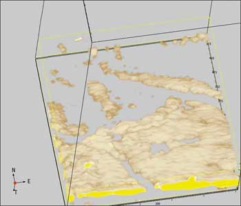
Seismic data over the study area was decomposed into smaller, 5-Hz bandwidths. Spectral decomposition amplitude around 19 Hz is extracted from the mapped horizon, resulting in the spatial expression of the attribute. With the ability to display, in this case, just the 19-Hz attribute of the 3D interval and filter out negative data values, the interpreter can easily identify three feeder channels from the northwest rather than one, and the two downdip channels now appear to be amalgamated, Fig. 3a. This resulting interpretation of deposition is radically different using dense 3D attributes rather than using sparse data such as well logs.
|
|
|
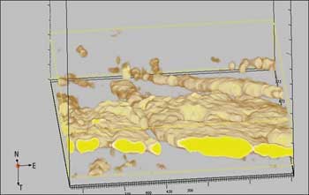
Fig. 3.a) The filtered spectral decomposition data around 19 Hz shows the three feeder channels from the northwest. b) A side view of the data illustrates the potential for five downdip lobes. c) Spectral decomposition attributes extracted from the time surface are shown. d) A graph of the spectral decomposition data against the net sands is overlain with a linear regression line showing the relationship between the two data sets. e) A calibrated attribute map represents the net sands between well control data.
|
|
By turning the 3D view to the southern side of the data, the reader can see that the amalgamated areas do display some indication of five lobes downdip, shown by the stronger yellow colors encased in brown in Fig. 3b.
Sophisticated software allows a horizon to be extracted, which enables a mapped surface to pick up points from a selected attribute in the seismic time samples of the mapped surface. Once extracted, the new attribute information is integrated with the net sand information from the well control data. The 19-Hz attribute extracted at the structural time is shown by Fig. 3c.
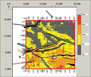
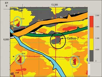
The next stage is to integrate well information with seismic attributes by graphing the net sand from each well log in the zone of interest and the associated spectral decomposition value at the well location. Figure 3d illustrates the relationship between the seismic and the well log values, showing a linear mathematical correlation. Using this new knowledge, the attributes on the map can be used in a linear fashion (Fig. 3e) to predict in undrilled areas the amount of net sands expected to be encountered. The color bar has been adjusted to show the background in gray; this color bar is similar to the amplitudes that were filtered out in the 3D opacity filtering in Figs. 3a and 3b.
The calibrated results in Fig. 3e show that there are three major feeder channels of 50-100-ft-thick channels elongated from a source in the northwest to the lobate deposition downdip, which is shown in yellow. The downdip deposition is up to 150-200 ft thick in areas.
Often deposition with large amounts of clastic sediment influx causes normal faulting as the sediments slump or fail while they reach an unstable thickness on dipping gradients, but in the study area these sediments show thicker deposition in the southern area and upthrown of the fault. This scenario indicates that the deposition was completed before the faulting. Counter-regional faults occur often with withdrawal of material (salt and sediments); however, a more regional data set would be needed to reconstruct a better interpretation of the underlying withdrawal. An interpreter could conclude that since both upthrown and downthrown wells are producing and the fault was post-deposition, the hydrocarbon most likely was in place after deposition and before faulting.
DEFINING ANOMALIES
Before interpreting an isopach map, the explorationist must understand the anomalies that exist in the attribute map.
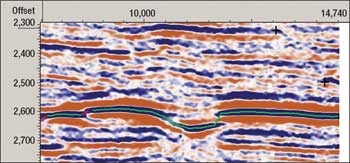
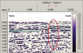
The first anomaly is the large dark area that is calibrated to an isopach of 50 ft or less in an area adjacent to the 150-200-ft isopach interval, Fig. 4a. This juxtaposition is interesting, so let us examine the original seismic through the anomaly indicated by the vertical red overlay, labeled Line 1. Figure 4b shows the anomaly in cross-section. The structure on seismic was interpreted as a graben, but does this really reflect the true structure?
|
|
|
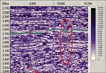
Fig. 4.a) The first anomaly of a low attribute value is shown next to a high attribute value. b) Reflectors show a possible graben structure. c) Instantaneous Q shows a frequency loss below the anomaly along with underlying compressed reflectors.
|
|
Calculating other attributes from the waveform can aid in the addition of information not readily seen in standard amplitude data. The attribute Q, a quality measure of the ratio of the seismic wave’s peak energy to its dissipated energy (or the frequency absorption of the data), indicates that below the structural graben, the underlying structure for about 800 ms of data seems to be buckled and distorted rather than a structural graben like the mapped horizon, Fig. 4c; in fact, contrary to the structural low, the underlying reflectors appear to indicate positive structures, as if in compression. Compression features that manifest themselves circularly on the map view (Fig. 4a) are areas of vertical gas migration, and thus the resulting waveform is distorted by the slower velocities of the gas surrounded by the normal velocities of the matrix. In conclusion, the interpreter finds that this area does not reflect the true structure, and the attributes are not correctly reflecting the values. This means the anomaly may have higher sand isopach than what is indicated by the seismic data, and that the structure is higher than currently mapped.
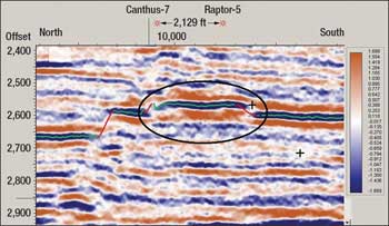
The second anomaly, to the west, is circled in Fig. 5a, a north-south seismic line corresponding to the red overlay labeled Line 2 in Fig 5b.
|
|
|
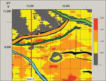
Fig. 5 a) A second anomaly of low attribute values is juxtaposed with areas of high attribute values. b) Seismic shows a regular and contiguous time structure. c) Instantaneous Q does not exhibit any anomalies. d) Log facies overlaid on the attribute map show that the area of interest is a region of little sand deposition.
|
|
It is important to note that the map in Fig. 5b indicates that the anomalous area is more regular and contiguous, and without the pronounced structural variations seen in the larger circular anomaly discussed above. Also, the reflections below the anomaly in Fig. 5a are parallel and do not indicate any underlying structural influence, in contrast to Fig. 4b. The attribute Q does not exhibit compressional buckling of the underlying data (Fig. 5c), as was seen in Fig. 4. Since there is no amplitude or structural variation, there should be an explanation other than seismic velocity distorted by gas.
Integrating the log facies for the downdip well Canthus-7 on top of the attribute shows the geology of the anomalous area to be a series of sands that are thining and fining upward. The well log information indicates that the color scale of about 50 ft or less of sand is a true representation of the seismic attribute data, and is not a geophysical anomaly but an area of little deposition, Fig. 5d. The next stage, now that the structure and the stratigraphy are understood, would be to prospect in the area for development opportunities.
ASSESSING STRUCTURAL RISK
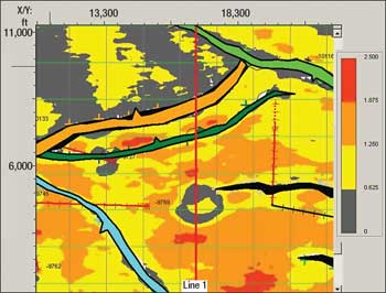
There exists a prospective development area updip of the Canthus-7 well containing 100 acres of closure, which is colored yellow and hachured in Fig. 6a. Examination of the area’s geology and integration of the well information and seismic attributes indicate that a well should encounter sand thickness in the range of 100-150 ft. Nonetheless, the trapping risk represented by the faults should be evaluated as well, prior to drilling.
|
|
|
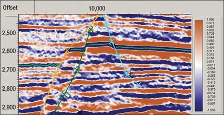
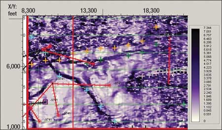
Fig. 6 a) An updip prospective area of current drilling is shown. b) The north-south seismic line shows the three trapping faults: green, orange and the questionable blue fault. c) A seismic time slice of the dip-of-maximum-similarity attribute shows the continuous blue fault connecting and trapping into the orange fault.
|
|
A north-south-oriented seismic line in Fig. 6b intersects the three trapping faults: orange, green and light blue. There is no dispute that the orange and green faults are present, as they are associated with displacements in the seismic of 30-50 ms of separation. The light blue fault is questionable in that the fault could be present below the resolution of the seismic data, or the seismic reflection could be a structural gradient. Defining the difference between a fault and a structural gradient change is critical to the entrapment of any potential hydrocarbons updip of the Canthus-7 well.
Dip of Maximum Similarity (DMS) is a semblance attribute comparing adjacent traces geometrically. Calculating this attribute will show edges in seismic data where data is dissimilar and/or similar. Figure 6c is a time slice at the objective level using DMS. The darker attribute areas represent regions that are not similar, and align along the plane of the light blue fault, which is indicated by light blue “X” symbols. These symbols mark locations where the interpretation was conducted in both an inline and a cross-line fashion. Using an attribute other than amplitude assures the interpreter that the fault in question is actually present and is likely a trapping fault. Hence, the addition of DMS helped reduce the structural risk for a trapping fault.
Now with the trapping fault confirmed, the development acreage is determined to be 100 acres of closure updip of Canthus-7, and the drill should encounter 100-150 ft in the closure.
CONCLUSION
Integration of the seismic attributes (amplitude, spectral decomposition, dip of maximum similarity, and instantaneous Q) with well log information helps the explorationist reduce structural and stratigraphic risk and determine the phase of the data and the pay signature before drilling. Understanding risk prior to drilling will make exploitation and development portfolios more successful. 
|
THE AUTHORS
|
|
|
K. Rene Mott is a Senior Technical Adviser at Seismic Micro-Technology Inc. She holds a BS degree in geophysics from Texas A&M University and an MS degree in seismology from the University of Texas-Dallas. She worked for Unocal for 9 years as an explorationist; at Maxis Energy in Dallas for 5 years as an explorationist; and for four other independent companies in exploitation and development before joining SMT in 1999 as Technical Services Manager.
|
|
| |
Veronica Hunt is the Marketing and Sales Manager for Fairfield’s non-exclusive 3D seismic data. She earned an MS degree in Marine Science from Long Island University. She joined Fairfield Industries in 1980 and has been involved in high-resolution studies and onshore/offshore acquisition of both 2D and 3D programs. She is involved with the IAGC on the data licensing committee and is a member of SEG.
|
|
|


