The benefits of pumping slowly

Matching the pumping capacity to the reservoir inflow can greatly increase run life while maintaining maximum liquid production.

Paul M. Bommer, University of Texas at Austin; and David Shrauner, Zachry Exploration Ltd.

One of the largest operating costs, and often the largest, associated with sucker rod pumping is the expense of pulling and repairing the rods, pump and tubing. Many wells are pulled for repairs so often that they are marginally economic. This problem is made worse by the days of lost production associated with the downtime. Pumping slowly can resolve these difficulties, making marginal wells economic over a long period of time.

CUSTOMARY PRACTICE

As reservoirs deplete, there comes a time when a sucker rod pump installation can lift more liquid than the reservoir can deliver. Excess pumping capacity results in excessive wear from shock loads caused by fluid pound, unnecessary friction and stress fluctuations.

The customary method of limiting this damage is to pump intermittently. This is done by placing the unit on a time clock or by installing a pump-off controller.

Both methods have at least four drawbacks:

1. Intermittent pumping changes the frequency, but not the pumping speed. When the unit comes back on, the loads associated with motion and fluid pound reoccur.

2. While the pumping unit is off, the reservoir continues to flow liquid into the wellbore. This flow builds a liquid level in the casing, which creates backpressure on the producing formation. Optimizing flow requires minimizing backpressure, which is achieved by keeping the liquid column in the casing as small as possible.

3. Starting the unit from a dead stop requires the maximum power usage. The start phase is also a significant shock on the pumping unit, rods and pump.

4. If the well produces any solids, downtime allows the solids to settle. This will increase the frequency of stuck plungers.

Therefore, the customary methods cannot eliminate all the shocks, unnecessary pump cycles and unnecessary power use, nor can they provide the minimum backpressure against the reservoir at all times.

SLOW-SPEED SOLUTION

As pump speed increases, so does the number of cycles, which causes the rods to reach their fatigue limit more quickly. The number of pumping cycles and the stresses caused by motion can be minimized if the unit is pumped as slowly as possible, using the longest stroke possible, to produce the maximum flowrate the reservoir can deliver. Using this method produces longer run times.

A sucker rod subjected to a fluctuating load can tolerate only a given number of cycles before the rod fails. Goodman’s work considered steel specimens that were cycled to a maximum stress (_max) and then back to the initial minimum stress (_min).¹ He considered 4 million cycles before failure to be an “infinite life.” Other researchers define infinite life as between 1 million and 10 million cycles.²

Figure 1 shows a modified Goodman diagram that is used for API sucker rod analysis.³ This diagram shows stress as a fraction of a rod’s minimum tensile strength (T_min). The API maximum line is below the maximum suggested by Goodman, making the range of allowable stresses smaller than that allowed by Goodman. The intercept of the maximum stress line at zero minimum stress is the rod’s fatigue strength, and is related to the number of cycles to failure.2 Goodman’s experimental correlation has a fatigue strength of one-half the minimum tensile strength and was for 4 million cycles.

The API modification of Goodman’s diagram has a fatigue strength equal to one-quarter of the minimum tensile strength, and the calculated number of cycles to failure is on the order of 10 million. A rod will tolerate more cycles if the required fatigue strength is a smaller fraction of the rod’s tensile strength. In fact, the expected life (Nf) is an exponential function of fatigue strength (Sf) as shown by Eq. 1, where a and b are properties of the rod.2 The rod properties used for this article are shown in Table 1.

TABLE 1. Rod properties

It is important to note that Fig. 1 only works for fluctuations in tension. A rod with the maximum load in tension and the minimum load in compression will experience greater fatigue than a rod with the same maximum load in tension and the minimum load kept in tension, and will thus have a shorter life.

Fig. 1. A modified Goodman diagram is used for API sucker rod analysis.

The API maximum stress line is described by:

It is customary to reduce the maximum allowed stress by a service factor that depends on the corrosiveness of the produced fluid and whether it is successfully inhibited. For a given minimum stress, any maximum stress that plots on or below the API maximum line is considered a safe fluctuation, when adjusted by the appropriate service factor. The further that a maximum stress falls below the API maximum allowed, the longer the service life will be. Slower pumping produces a smaller maximum stress, but also a larger minimum stress as both friction and acceleration loads are reduced, resulting in a smaller stress fluctuation. The number of allowed cycles increases because the stress fluctuation now falls below the original and has a smaller fatigue strength, as shown by Eq. 1.

A sucker rod string will be subjected to a maximum load during the upstroke and a minimum load during the downstroke. This is shown on the ideal-surface dynamometer card of Fig. 2. The parallelogram shape of the ideal card is the result of rod stretch.

Fig. 2. The ideal-surface dynamometer card shows one stress fluctuation per cycle.

Ideally, the rods experience one stress fluctuation per cycle. A stress fluctuation is when a load changes both magnitude and direction. For the ideal shape of Fig. 2, one stress fluctuation is created by raising the rods to a maximum load during the upstroke and lowering them to a minimum load during the downstroke. There often are many smaller load direction changes during a stroke that increase the number of stress fluctuations per cycle. Figure 3 superimposes the actual surface dynamometer card on the ideal card, showing several minor load fluctuations in addition to the major fluctuation caused by the maximum and the minimum loads. The minor fluctuations are more easily characterized if the dynamometer card is shown as a strip beginning at the start of the upstroke and finishing at the end of the downstroke, Fig. 4.

Fig. 3. Superimposing the actual initial surface dynamometer card for Example 1 on the ideal card shows several load fluctuations in addition to the major fluctuation caused by the maximum and the minimum loads.

Fig. 4. Plotting the initial dynamometer card for Example 1 as a load strip beginning at the start of the upstroke and finishing at the end of the downstroke shows that four stress fluctuations occur in one cycle.

The effect of minor fluctuations on rod life can be estimated using the Palmgren-Miner Rule:²

Figure 4 shows that all the fluctuations occur during one cycle, so in Eq. 3, n_i (the number of cycles at stress level ) = 1. The number of cycles associated with each fluctuation (N_f) is a function of the fatigue strength line upon which the fluctuation falls. D is the accumulated damage to failure; in a perfect environment, D = 1. The service factor (SF) allows for a corrosive environment and is generally taken as a fraction less than 1. For any fluctuation, the fatigue strength can be predicted using Eq. 2 and the accompanying fatigue life can be predicted using Eq. 1. Finally, the total expected life of the rod (N_T) can be estimated using Eq. 3.

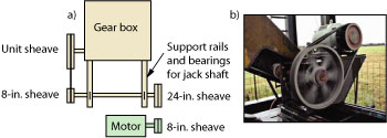
If the pump can lift more liquid than the reservoir can deliver, it is possible to reduce the speed of a unit such that the lift capacity closely matches the reservoir’s production rate. The necessary speed reduction can be achieved by replacing the unit or prime mover sheave or both. Even slower pumping can be achieved by using a second speed reducer known as a jack shaft, which fits between the prime mover and the gear box.

Fig. 5. a) A jack shaft schematic and b) a prefabricated unit with the belt guard removed for viewing.

A jack shaft is a shaft mounted on two bearings that have an input and an output sheave. The input sheave is attached to the prime mover sheave with a power belt; the output sheave is similarly attached to the pumping unit gear box sheave, Fig. 5. The speed of the pumping unit with a jack shaft, in strokes per minute (spm), can be calculated by:

where:

• N_pm = prime mover speed (rpm)
• d_jsi = pitch diameter of the jack shaft input sheave (in.)
• d_jso = pitch diameter of the jack shaft output sheave (in.)
• d_pm = pitch diameter of the prime mover sheave (in.)
• d_u = pitch diameter of the pumping unit sheave (in.)
• Z = pumping unit gear box ratio (revolutions/stroke).

Generally, the cost of the installed jack shaft is less than the cost of one tubing-pulling job. In our experience, at slow speeds the gear box requires no modification to ensure proper gear lubrication.

RESULTS

Two case histories are presented to demonstrate the utility of pumping slowly. When correctly designed, slow pumping will always produce results similar to these examples.

Example 1: Winkler County, Texas. This well was pumping from a depth of 3,210 ft at 13.5 spm. The rods had parted five times in 24 months. Figure 4 shows the load strip for one cycle. The pump barrel is filling about 65% on each stroke, and the load strip indicates four fluctuations per stroke. Table 2 shows the loads and stresses for each fluctuation. The peak polished rod load and the minimum polished rod load are the first fluctuation. Using Eq. 3 with a service factor of 1, these values result in a theoretical rod life of 512 million cycles.

TABLE 2. Initial loads and stresses for Example 1

The unit was slowed to 7.5 spm. Figure 6 shows the load strip chart at the slower speed. The loads and stresses for each fluctuation (Table 3) result in a theoretical rod life of 10.44 billion cycles, a 20-fold increase over the theoretical life at the original pumping speed.

TABLE 3. Loads and stresses for Example 1 at reduced pump speed

Fig. 6. The dynamometer card for Example 1 after the pump has been slowed is plotted as a load strip for a single stroke.

The unit ran for three years without a pulling job-a 7.5-fold increase in run time. By slowing to 7.5 spm, the unit lifts 36,615 tons/day less weight and requires 8 hp less power.

Example 2: Gonzales County, Texas. This well was pumping from 8,400 ft at 6.25 spm. The rods had parted six times in 34 months. The pump barrel is filling about 40% on each stroke, and the load strip for one cycle indicates five fluctuations per stroke, Fig. 7. Using Eq. 3, the loads and stresses for each fluctuation (Table 4) yield a theoretical rod life of 81 million cycles.

Fig. 7. The initial dynamometer card for Example 2 is plotted as a load strip for a single stroke.

TABLE 4. Initial loads and stresses for Example 2

This unit was slowed to 4 spm, Fig. 8. The loads and stresses for each fluctuation at this reduced pumping speed (Table 5) yield a theoretical rod life of 349 million cycles-a 4.3-fold increase in theoretical rod life. The unit ran for five years without a pulling job, 10 times as long as the average for the previous six pumps. At 4 spm, the unit lifts 20,140 tons/day less weight and requires 6 hp less power.

Fig. 8. The dynamometer card for Example 2 after the pump has been slowed is plotted as a load strip for a single stroke.

TABLE 5. Loads and stresses for Example 2 at reduced pump speed

The production rate for both examples remained the same after the pumping speed was slowed as before. In the event that the production rate drops after slowing, it indicates more pump slippage than previously thought. The solution is to speed the unit slightly until the original output is maintained.

The discussion to this point has focused on extending rod life by pumping more slowly, but pumping more slowly extends tubing and pump life as well.

DETERMINING MAXIMUM RATE

For sucker rod-pumped wells that have an excess pump capacity, it is usually obvious what the well will produce. If this is not so, the pumping unit can be run continuously until a daily rate is established. A representative dynamometer card will show how much the pump is filling on each stroke. Fluid levels can yield useful data, but they must be used carefully, because a small slug of fluid or foam in the annulus will appear as a fluid level and indicate a greater inflow from the reservoir than is actually present. However the initial estimate is made, it is excellent practice to check the final design using a dynamometer after the well has pumped for several days.

CONCLUSIONS

Matching the pumping capacity to the reservoir inflow is the key to maximum liquid production and long run life. For wells with excess pump capacity, the best way to achieve this is by slowing down the pumping rate. The smallest possible pumping speed to provide the required capacity will:

• Produce 100% of liquids available from the reservoir
• Reduce rod stress fluctuations and shock loads
• Cause the unit and rods to do the minimum work
• Use the minimum amount of power
• Keep the pump in motion to prevent solids from sticking the plunger
• Provide the longest run time possible
• Create the largest profit by maximizing production and minimizing pulling frequency.

Our experience with more than 500 sucker rod-pumped wells in four states has verified these claims.

Every sucker rod pump that has excess capacity should be slowed so as to pump continuously and match the daily flow from the reservoir. The well conditions after a change should be checked using dynamometer analysis.  

ACKNOWLEDGEMENT

This article was prepared from SWPCS 200701 presented at the Southwestern Petroleum Short Course held in Lubbock, Texas, April 23-24, 2007.

LITERATURE CITED

¹ Goodman, J., Mechanics Applied to Engineering, Longmans, Green and Co., London, 1914, pp. 631-636.
² Shigley, J. E., Mischke, C. R. and R. G. Budynas, Mechanical Engineering Design, 7th Ed., McGraw-Hill, New York, 2004, Ch. 7.
³ RP 11BR: Recommended Practice for Care & Handling of Sucker Rods, American Petroleum Institute, Dallas, 1989.