Production Technology

Conformance Engineering: A comprehensive review

Part 3: Proper solution is benefit analysis

David Smith, OXY Permian, Houston; and Bill Ott, Well Completion Technology, Houston

In Part 1, we covered basics of Conformance Diagnostics. Part 2 connected the problem to an effective solution. In this article, we review the proper elements of Benefit Analysis.

Although the elements of this review are very basic, they allow us to streamline the process and generate a simple, economic screening tool to more accurately show the true benefit. The thoughts and ideas presented are designed to assist you in working through the process of Conformance Engineering, and we hope they will be a catalyst for further discussion.

ANALYZING THE ECONOMIC BENEFIT

When considering all of the benefits from controlling unwanted water or gas, it is often difficult to generate a financial analysis that is simple, complete and yet accurate in its assessment. The method that follows generates economic benefit from conformance work that will simplify the analysis and incorporate more of the overall benefit than is usually considered.

This technique is similar to one used at Prudhoe Bay Alaska in the early 1990s, used to generate the expected benefit from Gas Shut Off (GSO) treatments. It has been modified here for use with Water Shut Off (WSO) treatments. When reviewing this methodology, please remember this analysis is only one way of approximating the benefit derived from conformance solutions. The terms and system designed below are set up to handle WSO or GSO treatments – including CO₂ – for oil production wells and/or injection patterns.

This method uses three elements to derive the “Equivalent Net Oil Benefit,” or E-NOB. “Equivalent” denotes conversion of the operating expense cost-savings element into an equivalent of oil production benefit. The term “Net” denotes a value that is the sum of both positive and potentially negative elements that combine to show the overall value.

The three elements are, Q_od (Direct Rate Benefit), Q_oid (Indirect Rate Benefit) and the Q_oes (Operating Expense Savings).

DIRECT RATE BENEFIT: Q_od

The first and easiest term to define is Q_od. This element is simply the increase or decrease in oil rate that is observed from a well or pattern. The equation for this term is:

This is only for the well or pattern treated. For injection-well treatments, this includes all affected producers. Generally, this is only for the immediate pattern, but may be modified based on performance. Another distinction between producing-well treatments and injection-well treatments is a time lag. Producer-well treatments show a rapid or immediate response to treatment. In injector treatments, the response is often delayed by several months before the impact is seen at the producers. Thus, with injector treatments, a time lag needs to be applied to the benefit.

INDIRECT RATE BENEFIT: Q_oid

The second term, Q_oid, requires the introduction of several new terms. The first is called the field’s “Facility Utilization Factor,” or F_uf. If you remove X total fluid rate from the facility system, you will, to some degree, replace a portion of that fluid rate with other production. Some portion of this freed-up facility capacity may be used, based on facility constraints and your ability to recognize and use it. This will be done either through 1) an active effort to maximize facility throughput by adding wells that are currently shut-in, or 2) by passive replacement, which is the result of the increasing drawdown on wells tied into the same system, due to a minor change in overall system pressure.

The combination of these two elements becomes the field and facility systems F_uf (or your ability to replace fluid). The units of this term are expressed as a fraction and must be estimated based on the overall facility optimization. Again, the F_uf is that fraction or portion of the total fluid rate that was removed from the system that you expect to replace.

The next term to define is the average WOR or GOR of the replacing fluid (RWOR or RGOR). When the field replaces X volume of the fluid that was removed from the system, what you are trying to define is the average WOR or GOR for that new fluid brought into the system. In some fields, you might assume that this value is the average field WOR or GOR. In general, this would be true if all of the replacement fluid is passive. This is the most optimistic value you should use.

A more conservative value to use is the marginal WOR or GOR, which can be defined as the threshold ratio at which you chose to shut wells in rather than produce them. This is only true where all fluid replacement comes from bringing on shut-in wells. This shut-in threshold is a more accurate value. The expected value for the replacing fluid will be some where between these two terms as used in the example. In general, if you are actively replacing the fluid, then F_uf should be high (>50%), in this case the WOR or GOR should be closer to the marginal value. If most of your fluid is passively replaced, then F_uf should be low (<30%) and the WOR or GOR should be closer to the field average.

The next term is the Q_fr (Total Fluid Rate Removed – for the limiting fluid). This can be simply defined as the total fluid rate before treatment minus the total fluid rate after treatment. For Water Shutoff (WSO):

Units are in bwpd, and only for the well or pattern treated.

For Gas Shutoff (GSO):

Units are in Mcf, and only for the well or pattern treated.

Now that all of the necessary elements are defined, the following equations generate the Indirect Oil Rate Benefit, Q_oid:

For WSO:

For GSO (or CO₂):

The resulting units are in bopd.

OPERATING EXPENSE SAVINGS: Q_oes

The third term, Q_oes, required to generate the total Solution Benefit (SB), comes from the Operating Expense Savings that is generated by not having to handle and re-inject the water or gas that is not replaced by the system. This term, Q_nfr (Net Fluid Removed), is generated by:

For WSOs, this results in bwpd units; for GSOs, the result is in Mcfd.

The real key is to define the Cost of Handling the Undesired Fluid, or P_uf. This term requires some extensive background and knowledge of your field operating expenses, and may not be readily available. Even if no accurate value can be generated, you should be able to generate a conservative estimate. That value can then be used to further your understanding of the total SB generated by the treatment. The units of this term should be in $/bbl for water or $/Mcf for gas/CO₂. Remember, when you estimate or generate this value, be conservative; only generate the cost that is directly variable and truly depends on handling of that fluid volume.

As an example, the cost of generating the horsepower to lift a barrel of water, plus the cost of treating that water with corrosion inhibitors and/or de-emulsifiers, and finally the cost to re-inject a barrel of water to replace the voidage. All of these terms are the true incremental costs associated with handling each barrel of water. Again, to be conservative, do not include all the fixed costs that are associated with maintaining the overall system or that cannot be eliminated just because a small volume of the whole is removed from the process.

Finally, to make these units equivalent to the other terms, you divide this dollar-cost savings benefit by the revenue generated from the production of a bbl of oil. We define this term as the N$_PBO (Net $ per bbl of oil) and express it:

Some might argue that you should also subtract items like working interest, or operating expenses. But remember, this method equates the cost savings generated by eliminating the cost of handling undesired fluid; this savings will come directly out of the Net Revenue excluding only severance taxes, royalties, and tariffs. Thus, Q_oes is defined:

We want to emphasize that this technique is only used to generate a combined net benefit on like terms. By doing this, it gives us a relative understanding of the impact of Opex Savings, while maintaining the real dollar value of the overall program. In addition, this method allows incorporation of an automatic reduction in the benefit over time through the decline rate. Later on, we will describe using this decline factor to project a deterioration of these benefits, which includes a reduction in the Opex Savings.

TOTAL SOLUTION BENEFIT: Q_sb

Now that all the necessary elements of the SB have been defined, the final equation is a simple summation, whose units can now be combined to define an E-NOB or Equivalent Net Oil Benefit:

Where ebopd is the operating expense in equivalent net bopd.

SOLUTION BENEFIT EXAMPLE:

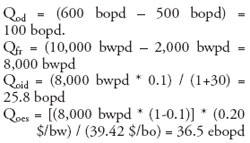
Table 1 is an example of how the SB can be calculated. This case is a WSO treatment, and the values are made up, but are typical of cases we have seen.

Substituting the table vales, we have:

TABLE 1. Typical values for Solution Benefit calculation, WSO treatment.

Thus, the E – NOB of executing this treatment is:

PROJECTING TOTAL BENEFIT 

We can project a total economic benefit from the E – NOB by monitoring or projecting the production history over the next several months and years to establish the benefit decline. This is required to understand the true economic benefit of the solution.

However, in many cases, this total benefit decline rate is unknown, and must be estimated. To estimate the overall decline rate from the cumulative benefit without field data can be difficult. A good first estimate is to double the normal field decline rate. This is done by assuming an additional decline rate for the SB that is equal to the field decline rate. This additional decline rate is normally expected for the Q_oid and Q_oes elements of the total Q_sb.

To simplify calculation, we are also going to assume this double decline rate for Q_od, but remember, this is a very conservative assumption. We can then calculate the cumulative additional E-NOB generated by the solution, until it returns to the original well rate or, we can truncate the benefit at 10 yrs. An example of this technique, based on a normal well decline rate of 10%/year and an additional decline rate for the SB of 10%/year, would yield an expected cumulative E-NOB of ~ 255,600 bo. Remember, this is an equivalent value and can not be taken as reserves.

A conservative approach used at Prudhoe Bay is crediting the solution with only that portion of the cumulative benefit which was above the original rate of the well. In this example, that value was ~ 66,000 bo.

Remember, the best way to estimate these values is to establish actual field data trends. Without field data, it is important to run sensitivities. This is easily done by entering the formulas into a spreadsheet and changing the additional decline rates to match what you see in the field. Using these techniques you will be able to estimate the cumulative benefits of future work with much greater confidence in their overall benefit.

APPLICATION OF ECONOMICS

Up to this point, we have only discussed the elements to estimate the benefit generated from Conformance Solutions. In order to show the value that is generated, we need to incorporate the cost of doing the problem diagnostics, and the work completed to generate and execute the solution. Using these costs, the Qsb flow stream in E-NOB and the N$_PBO defined earlier, we can generate an incremental cash flow stream that will provide additional insight into the potential value that can be created.

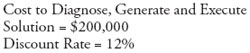
The final elements needed are the desired discount rate and a price forecast for oil. Given a typical discount rate of 12% and using a flat Net Revenue per bbl (N$_PBO), economic values can be calculated:

Using these values and the rate stream generated from the example, the estimated overall value generated is:

As a whole, this system is still rather conservative, but it provides some simple factors that can be adjusted and tested for sensitivity. In this way, a more complete view can be generated of the expected results and the key factors to the overall economic success of the project, Fig. 1.

Fig. 1. Representation of the benefit, plotted with treatment in the sixth month and first benefit in the seventh month.

The program that generates this analysis is currently available only within Occidental Petroleum. However, in the future, Halliburton is working on a Website where these same basic screening terms and calculations will be available; a Beta version is being tested. This analysis is only built for initial screening criteria and does not incorporate all tax implications, etc. You should be able to use these methods to quickly screen the value of conformance efforts.

LEARNING FROM THE PROCESS

In Part 1, we talked about the need to understand the problem before attempting solutions. Experience has shown that, when we fail, it is generally because we misunderstood the problem, and not that the tool or technique failed. There are many famous quotes that relate experience, failure and success, and most of them are very applicable to Conformance Engineering work:

What we would like to leave you with, is that each failure in conformance efforts has the ability to teach something more about your problems. Remember, understanding the problem is the key to solving it, and the only time you have truly failed is when you have given up on learning from the experience. You may not be able to completely control your conformance issues, but experience has shown that, persistent effort and a willingness to improve from the process will ultimately lead to an ability to solve conformance problems, enough to create economic success for your efforts. 

THE AUTHORS
	David Smith has been the senior conformance engineering advisor for OXY Permian for the last four years. He now works as an in-house consultant for conformance solutions that are beyond the scope of normal operations. Smith can be reached at david_smith@oxy.com.
	William K. (Bill) Ott is founder (1986) and president of Well Completion Technology, a Houston-based international petroleum industry consulting and training firm. Previously, he was training manager for Triton Engineering Services, and division engineer for Halliburton’s Far East region. Mr. Ott received his BS degree in chemical engineering from the University of Missouri. He is a registered professional engineer in Texas and Missouri.