Reservoir Characterization

A method to estimate permeability on uncored wells

The method, based on cores and log data, has been shown to outperform standard-regression techniques, as well as the hydraulic-flow-unit approach.

Pablo E. Lacentre, Repsol-YPF; and Pablo M. Carrica, University of Iowa

Reservoir simulation studies require good knowledge of permeabilities, but reliable measurements are only available from laboratory core tests. These are usually taken from a small percentage of wells. Frequently, this information is extrapolated to calculate permeabilities over the field, but insufficient data points usually cause unreliable predictions. This article proposes a method to estimate formation permeabilities from standard well logs and core data. The method should be applicable to any reservoir as long as sufficient core and log data are available. The method assumes that the Carman-Kozeny equation holds for the reservoir rocks, which is a fairly reasonable assumption, and that the available well logs contain intrinsic information on tortuosity, sand size distribution, cementing characteristics, etc., which ultimately determine flow performance.

This hypothesis is usually strong because the available logs are not able to fully read the physical phenomena that cover the complex dynamics of flow through reservoir rocks. The method was tested in a sandstone formation in Chihuido de la Salina, Neuquen basin, Argentina. Some core data points were not used to train the neural network and were subsequently useful for validation and comparison. In spite of certain drawbacks, the method was shown to outperform both standard-regression and hydraulic-flow-unit approaches.

INTRODUCTION

Accurate determination of permeability is paramount because it affects the economy of the development and operation of a field. It influences production rates, ultimate recovery, well placement, pressure and fluid contacts evolution, etc. The most reliable local permeability data are from lab analysis of cores. Extensive coring is very expensive and is only reasonable in very limited cases. In general, core data are available only from some wells in the field, and for some intervals in each cored well. Then the permeability of the whole field is estimated from this sparse information. This frequently results in a lack of statistics that causes poor prediction capabilities.

The authors begin with an approach already explored by several researchers,^1,2 consisting of finding a relationship between diverse well log data and the core permeabilities. Typical, classic methodologies are the logk vs.f transform³ or, more recently, the use of the Flow Zone Indicator (FZI) technique.⁴ There are also correlations to predict permeability based on porosity and lithologic volumes,³ thus allowing a permeability profile to be obtained. These predicted permeability “logs” can be calibrated to fit pressure-transient analysis tests,⁶ usually the most widely accepted integral permeability measurements.

A method is presented to obtain permeabilities from all available well logs. The method takes advantage of modern mathematical tools that have proven to be effective in other fields of science and engineering, including neural networks, cluster analysis, principal components, etc. The method was tested and compared against independent core data, correlations, and the FZI method.

THEORY

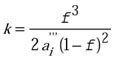
As early as 1927, Kozeny¹¹ proposed a model relating porosity – a log measurable property – and permeability. The original model was slightly modified by Carman in 1938 to yield the Carman-Kozeny equation:⁷

(1)

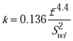
where a_i^''' is the fluid/ rock interfacial area density andf is the porosity. An approach to account for the irreducible water saturation is the Timur equation:¹

(2)

Other, similar correlations are available in the literature. These empirical correlations lack the information necessary to describe flow on pore throats and, consequently, fail to predict permeability with the exception of a few cases.

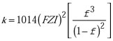
In view of the explained problems, some attempts have been made to use different well logs that, hopefully, contain enough information to describe flow characteristics through pore throats. As this relationship between well logs and permeability is not known a priori, some statistical analysis of the data is necessary to extract useful information from it. Conventional statistical regression has been done parametrically in the past, using linear or nonlinear models. A widely used approach is the Flow Units Method.^4,7,8 In this method, permeability is related to porosity and the FZI as:

(3)

In this equation, the FZI must be correlated to wireline log responses for known core permeability and porosity data. As a first step, the FZI is classified using some sort of cluster analysis, such as a histogram analysis, probability plot or other.⁷ Then the FZI must be predicted in wells where only logs are available.

The introduction of non-parametric methods has allowed a better description of permeability. Techniques such as Alternating Conditional Expectations (ACE) and Neural Networks (NNET) have been used.⁹ In this work, we use the NNET method to directly predict permeabilities.

METHODOLOGY

Preliminary data analysis. The method was applied to three independent blocks at Chihuido de la Salina field: Rincón de Correa, Escama Superior and Escama Intermedia. In this region, reservoir is fluvial in origin, consisting of medium-to-coarse grain quartz sandstone and a small proportion of argillaceous matrix. It can be divided into six vertical sequences with good lateral continuity. The upper layer, denominated TAS, has shale volumes between 30% and 50% and porosities less than 10%. The five lower layers (TP1 to TP5) are productive and average 18% porosity and less than 30% shale volume. Typical permeabilities are about 100 mD, although there is a heterogeneous distribution ranging from 0.1 to 1,000 mD.

Four wells in the field were cored, totaling 130 m. There was good correlation between the porosity and density logs, and the core values. Only well logs that were available in all wells were used in the analysis: GR, NPHI (thermal neutron porosity), PEF (photoelectric factor), RHOB (bulk density) and LLS (laterolog shallow resistivity). In addition, a petrophysical interpretation with Schlumberger's Petroview Plus 10 was performed to obtain the lithologic volumes of dolomite, illite and quartz. Fig. 1 shows the histogram of the volumes of dolomite and shale on the sands under study. A plot of the log( k) vs.f and a typical linear regression is shown in Fig. 2, for different lithologies. It can be seen that the correlation is poor, even after a classification in lithofacies.

Fig. 1. Histogram of volume fractions of dolomite and shales.

Fig. 2. Log(k) vs. porosity plot classified by lithofacies.

Fig. 3 shows a comparison of the linear regression of Fig. 2, the method of Herron, and the core measurements for one well (ChLSSEI.x-1001). Even though the qualitative trend is appropriate, both methods are in gross error.

Fig. 3. Permeability vs. depth for a cored well comparing the classical methods (log(k) vs. f and Herron) with the core data.

The well logs and cores were normalized in depth to properly compare each of the layers: TAS and TP1 through TP5. Then the experimental FZI was calculated from the core data, according to Eq. (3). The distribution of the log 10 (FZI) is shown in Fig. 4. Each of the peaks in the distribution should represent a group or cluster with gaussian distribution, since both log(k) and log(f) have normal distributions.¹¹ However, the group classification is not apparent since there is a strong overlapping. To identify the cluster, a self-organized neural network was used, with a competitive input layer.¹² The structure of these neural networks has been specifically designed for cluster analysis, and allowed the identification of nine hydraulic units, as shown in Fig. 4.

Fig. 4. Histogram of log 10 (FZI) and Gaussian fit.

Core permeability as a function of effective porosity for the cored wells is shown in Fig. 5. The data was separated in hydraulic units and Eq. (3) was also plotted for the average FZI from Fig. 4. Notice that there is still a substantial scatter of the data in each hydraulic unit that can reach variations of one order of magnitude at a given porosity.

Fig. 5. Permeability as a function of porosity for each hydraulic unit.

Prediction of permeability with neural networks. In this new method, we attempt a direct mapping between well log data and core data for a given set of experimental points. From the physical standpoint, there is no theoretical reason whatsoever that guarantees a connection between the permeability, a purely dynamic parameter, and the static variables measured by well logs. If such a relationship exists, we will find it through mathematical analysis, not through geological or physical interpretation. Even though a link usually exists between well logs and permeability, it is extremely difficult to formulate an analytical function that could describe this link; therefore, our method can be categorized as a blind.

Neural networks with supervised learning is an ideal tool for this type of problem. A widely used structure is the backpropagation network, shown schematically in Fig. 6.

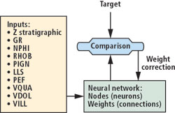Fig. 6. Schematic of the use of the neural network in this work.

In this work, we used different backpropagation network models, all of them with an input layer where all the well log data are introduced, a single hidden layer and an output layer with one neuron whose response is compared against the core data. This comparison results in an error in the prediction of the network, and the weights are corrected in order to minimize the error. The process is repeated for each depth, choosing the depths in a random manner. The network training is finished when the error falls below 1% or when the network stops learning from the data set. This condition is determined from a parallel set of data used to monitor the learning process of the network.

A flowchart of the methodology is shown in Fig. 7. As a first step, the data set was divided into two sets, one for the network training and the second for training validation. The validation set was taken from nine data points, one from each of the above mentioned flow zones. This procedure was favored instead of taking a cored well, because in this way, all flow zones are equally represented and the number of data points used for training are maximized, reducing the ratio of parameters to adjust (weights) to data points. In this work, this ratio is less than 0.3. As a general rule, the lower this number, the more “predictive” will be the neural network.

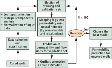Fig. 7. Flowchart of the methodology and data analysis processes.

The set of logs Z_strat, VDOL, VILL, VQUA, PIGN, GR, NPHI, PEF, RHOB and LLS were used as inputs for the network. Each of these records was normalized, subtracting the mean and dividing by the standard deviation. The use of 10 logs simultaneously forces too many neurons in the input and hidden layers, increasing the ratio of weights to data points. This results in too many degrees of freedom. Although this would improve the capability of the network to fit any function, it would also cause poor prediction capabilities under new inputs.

To address the problem, an analysis of principal components was performed for the data set. The technique considers that each well log is a vector, then a base of orthonormal vectors is made of linear combinations of them, which assures no correlation between these new elements. Then the importance of each of these new vectors in the original set of data is determined, evaluating the contribution of each of the principal components (the orthonormal vectors) to the variance in the data set. Fig. 8 shows the contribution of each principal component. It can be seen that 90% of the information is within the first four principal components, while 99% of the information is contained by the first seven principal components. This allowed us to choose between four and seven neurons in the input layer.

Fig. 8. Fractional contribution of each principal component to the total variance in the data set.

The training process was made by feeding the logarithm of the core-derived permeabilities, at the output layer. Direct use of permeability results in a lack of sensitivity to small values. Several models with different inputs, different neurons at the hidden layer, different weighting initialization and sets of training data were analyzed. The number of neurons at the input layer varies from four to seven, as already mentioned, and the number of neurons at the hidden layer varies from half to twice the number of neurons at the input layer. The initialization of weights is random and different for each model.

The Levenberg-Marquardt algorithm¹³ was used because it has a rate of convergence 10 times faster than the classic method of the descendent gradient. The training process of the network must be supervised to avoid the convergence to a particular solution (local minimum). Fifty training processes were performed for each model, initialized with different weights, and randomly chosen different points for the training and the validation sets. The predictions of the different models were compared against the core data for validation and the model with the least error in all flow zones was finally chosen.

Fig. 9 shows the convergence of the error for the training process of the neural network. When the difference between the training and the validation sets starts to increase, the training process is stopped, and it is assumed that the network cannot learn anymore from the data set provided. Then a new network configuration is analyzed.

Fig. 9. Training errors of the neural network for the training, test and validation data sets.

In Fig. 10, the correlation between the core data of permeability and the values predicted by the network for the selected model is shown. The measured points are those selected to evaluate the predictive power of the method and not those used to train the network. Notice the good correlation coefficient obtained.

Fig. 10. Correlation between the core permeability and the prediction of the neural network for a data set chosen randomly and not used for the training process of the network.

A comparison of the predictions and the measured values of the permeabilities and the flow zone indicator, as a function of the stratigraphic position inside the different layers, is shown in Fig. 11. The ordinates axis legend shows the different layers, 0 for the TAS, 1 for TP1, etc.

Fig. 11. Permeability and FZI, predicted and measured, as a function of the stratigraphic position for the same data set in Fig. 10.

As a final test, the predicted and measured permeabilities and FZI are shown for the cored interval in Well ChLSSEI.x-1001. Fig. 12 shows the correlation between the core permeability and the predicted permeability, while Fig. 13 shows the logs as a function of measured depth, adding the predictions by the method of Herron.⁵

Fig. 12. Correlation between the core permeability and the prediction of the neural network for Well ChLSSEI.

Fig. 13. Permeability and FZI logs for Well ChLSSEI. The blue line shows the predictions using the method of Herron.5

In the next section, we compare our method with the widely used method of the flow zones.^4,7 We will show that the method presented in this work is a generalization of the method of the FZI, and that it can solve many of the shortcomings and limitations of it.

FLOW ZONE METHOD

This method attempts to identify the flow zone indicator in uncored wells using log records. The first part of the analysis is based on the data processing already explained.

Once the flow zone indicator has been determined from the core data, a relationship between this FZI and the well logs must be obtained. Several methods have been proposed to this end, some based on classification in lithofacies and electrofacies.⁹ As already mentioned, the relationship between the different well logs, measuring static parameters and the permeability is not known. One of the most successful techniques to allocate the discrete FZI values to a set of measured values (well logs) is Discriminant Analysis. Given a set of n-dimensional vectors and n numbers indicating which group the vectors belong to, we want to classify a set of similar vectors.

In our case, each vector is a measurement at a given depth of the cored wells, and the vector values are the values of the n available well log curves. The number of flow zones n is nine and, therefore, each vector is assigned a number between one and nine. The uncored wells result in vectors we want to classify. In the method of discriminant analysis, the distance between each of the unclassified vectors and the measured (classified) vectors of each of the n groups is computed. Then the vector is assigned to the group with the lowest distance. This distance can be calculated using different metrics. In this work, we used Mahalanobis metrics, a cuadratic form that uses the correlation matrix between the data.¹⁴

The method was validated, separating 10 random core values from each group. The rest of the core data was classified as already described, and the validation set was then predicted and compared against the actual FZI at which each of the core points belonged. The validation data set was randomly varied in a Monte Carlo run and, thus, the overall performance of the method tested. The symmetric results showed that there was no over- or under-estimating trend, although only 52% of the data points were predicted within the actual or adjacent flow zone. Also, there was little or no correlation between the flow zones and the classification in groups made with well logs.

The prediction made for the validation data set was compared against the core FZI data from Eq. (3). The comparison is shown in Fig. 14 for randomly chosen data from different wells and flow zones. Fig. 15 shows the result for Well ChLSSEI.x-1001 and is compared against the method of Herron. Though the prediction is acceptable for most applications, the method fails to follow the strongest permeability variations. As shown in Fig. 16, the correlation coefficient for the validation dataset was 0.732, better than the straight prediction by a porosity-permeability correlation, but worse than the neural network method.

Fig. 14. Comparison between the core data and the FZI-predicted permeability values for a randomly chosen set of samples, as a function of the relative depth to the formation layers.

Fig. 15. FZI-prediction of the permeability for Well ChLSSEI against core data and the Herron method.

Fig. 16. Measured and FZI-predicted permeability crossplot for the validation data set: better than by a porosity-permeability correlation, but worse than the neural network method.

The sources of error in this method are mainly two: a) discrete values of the continuous variable FZI used in Eq. (3); and b) the mapping method has errors, the most important is that there does not always exist an acceptable correlation between the well logs and flow units.

In view of the previous analysis, we conclude that it is, in general, not convenient to perform a discretization in flow zones and/or electrofacies, because there is little correlation between these variables. The best that can be done is to find a continuous relationship between FZI and the well logs. Knowing the porosity, this is equivalent to mapping the permeability with the well logs, which is a more simple and effective approach.

CONCLUSION

A new method to estimate the absolute permeabilities from standard well logs (GR, LLS, RHOB, etc.) uses data analysis techniques that have been successful in other areas of science and engineering, such as neural network and principal-component analysis.

The results obtained were satisfactory and, in general, more precise than predictions with canonical methods. The results were compared against the classical linear mapping logarithm of permeability vs. porosity, the method of Herron and the more sophisticated method of flow zones, for a sandstone reservoir in Chihuido de la Salina field, Neuquén basin, Argentina. In all the tested cases, the method presented here outperformed the other methods, resulting in closer predictions to the core permeabilities, and allowed a better characterization of the hydraulic reservoir units. 

ACKNOWLEDGMENT

Part of this article has been possible thanks to the collaboration of the Finding Team, Faja Plegada Neuquina, of the Exploration and Production division at Repsol-YPF Latin-American.

REFERENCES

¹ Jing Long Lin and H. A. Salisch, “Determination from well logs of porosity and permeability in a heterogeneous reservoir,” SPE 28792, 1994.

² Johnson, W. W., “Permeability determination from well logs and core data,” SPE 27647, 1994.

³ Mattax, C. C. and R. L. Dalton, Reservoir simulation, SPE Monograph, Vol. 13, 1990.

⁴ Amaefule, J. O., M. Altunbay, D. Tiab, D. G. Kersey and D. K. Keelan, “Enhanced reservoir description: using core and log data to identify hydraulic flow units and predict permeability in uncored intervals/ wells,” SPE 26436, 1993.

⁵ Herron, M. M., “Estimating the intrinsic permeability of clastic sediments from geochemical data,” SPWLA 28th Annual Logging Symposium, 1987.

⁶ Bleckman, V., D. Díaz, P. M. Carrica, C. Corbett, B. Coca and U. Gómez, “Calibrating log-derived permeability data to pta for geostatistical integration into a fluid-flow simulation model,” SPE 69473, 2001.

⁷ Abbaszadeh, M., H. Fujii and F. Fujimoto, “Permeability prediction by hydraulic flow units – Theory and applications,” SPE 30158, 1995. Also in SPE Formation Evaluation, December 1996, p. 263.

⁸ Davies, D. K. and R. K. Vessell, “Flow unit characterization of a shallow shelf carbonate reservoir: North Robertson Unit, West Texas,” SPE 35433, 1996.

⁹ Lee, S. H. and A. Datta-Gupta, “Electrofacies characterization and permeability predictions in carbonate reservoirs: role of multivariate analysis and nonparametric regression,” SPE 56658, 1999.

¹⁰ Petroview Plus user guide. Trademark of Schlumberger.

¹¹ Kozeny, J., “Uber Kapillare Leitung des Wassers im Boden, Stizurgsberichte,” Royal Academy of Science, Vienna, proceedings Class I, V. 136, p. 271, 1927.

¹² Freeman, J. A. and D. M. Skapura, Redes Neuronales, Addison-Wesley, 1993.

¹³ Hagan, M. T. and M. Menhaj, “Training feedforward networks with the Maquardt algorithm,” IEEE Transactions on Neural Networks, Vols. 5, 6, 1994.

¹⁴ Mahalanobis, P. C., Proc. Of the Nat. Inst. of Sci., India, 1936, p. 12.