EXPLORATION / EXPLOITATION

Temperature anomaly mapping identifies subsurface hydrocarbons

Utilizing the fact that buried hydrocarbons alter the upward flow of heat through earth layers offers industry another valuable exploration tool

Lloyd Fons, President, Lloyd Fons Exploration, Inc., Houston

eat moving upward from deeper portions of the earth will arrive at various depths – and eventually to the surface – at different temperatures, depending on what type of materials (solids and fluids) it passes through. If a particular layer of subsurface material – say a hydrocarbon reservoir – has an insulating capability, the earth temperature below that layer will be higher, and temperature above it will be lower, than those below and above a noninsulating layer. Consequently, a temperature map will display a temperature anomaly above (and below) the hydrocarbon reservoir.

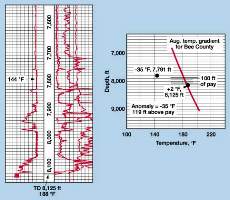
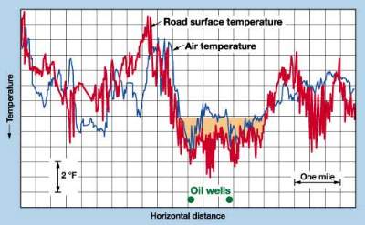
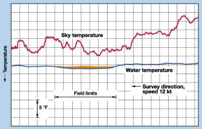
The following article discusses the concept of Temperature Anomaly Mapping (TAM), as it can be applied to locating subsurface hydrocarbons (insulating material), from temperature changes on the surface from one area to another. Below the surface, anomalies in the temperature gradient may be used to tell whether additional hydrocarbons exist below a particular well’s TD. The subject of TAM was introduced in a previous article;¹ and further case history applications will be presented at an October 2000 GCAGS meeting.²

Introduction, Theory

Although not perfect, this new hydrocarbon exploration / evaluation method may well be the most logical in the industry. It can be highly effective, and it appears to be fail-safe. The method finds hydrocarbons (quantitatively) with little reliance on other exploration data. Fundamentally, it entails construction and interpretation of temperature anomaly maps. Temperature profiles may be taken from: 1) bottomhole depths using BHT thermometers, Fig. 1; 2) earth surfaces by remote sensing, Fig. 2; and 3) near-surface air, and offshore water (at fixed depths below any thermocline), Fig. 3. Bottomhole temperature can identify deeper prospective pay zones and indicate when to terminate drilling.

Fig. 1. Bee County, Texas, Wilcox test. Negative 35°F anomaly indicates probable 75 ft, or more, of pay below first run TD. At final TD, positive anomaly of only 2°F suggests well should have been drilled deeper. Below pay zones exposed at present TD, one would expect a positive anomaly of about 40°F, indicating well should be drilled deeper before abandonment. Well flowed 5.8 MMcfd through perforations at 8,098 – 8,106 ft. Click for enlarged view

Fig. 2. Manistee County, Michigan, road surface temperature profile indicates productive pinnacle reef is 1.83 mi across and, apparently, a single well could have drained the structure. Two wells penetrated the reef. These surveys proved that pinnacle reefs are generally larger than previously thought and, in many instances, there is continuity of permeability between different pinnacles.

Fig. 3. Offshore temperature profile survey made at 14 mph, crossing Seabrook East field in Galveston Bay, Texas, perfectly delineated field without use of seismic, gravity, magnetic or oil-seep surveys. Depth of water varied from 10.5 to 11.5 ft. Survey was made in wintertime.

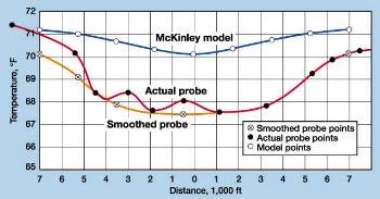
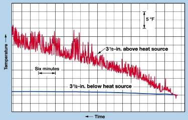
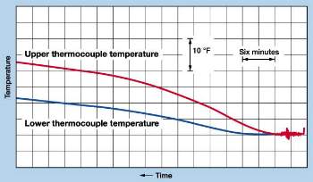
Creating five-foot-deep holes in unconsolidated sediments and measuring bottom temperature by thermocouple requires only about 20 minutes per station. To date, five-foot-depth temperature profiles have satisfactorily paralleled 100-ft-depth profiles, Fig. 4. This survey was completed in one day, by one person, with hand-carried equipment.

Fig. 4. Temperature cross-section of Friendswood field, Texas, using data taken from bottom of 11, 5-ft holes, compared to model by R. M. McKinley.

Infrared temperature surveys by either surface vehicle or airplane are limited by only the maximum speed of the survey vehicles and, occasionally, by adverse atmospheric conditions. Surveys by airplane have covered more than 600 mi, with answers obtained before breakfast.

The method will: 1) locate stratigraphic-trap reservoirs and predict reservoir shape and boundaries; 2) explore below the bottom of drilled holes; and 3) lower the cost of finding oil / gas by reducing or eliminating the need for seismic surveys and minimizing the risk of dry holes. It is simple, rapid, safe, environmentally compatible and inexpensive – permits are seldom required.

How It Works

Heat flows from within the earth to its surface, a process defined by the Second Law of Thermodynamics and Fourier’s Law. Hydrocarbons tend to be more insulative to heat flow than common earth materials. Hydrocarbons, in combination with connate water are, in turn, much more insulative to upward heat flow than hydrocarbons alone.

Because of these insulating properties, hydrocarbon-rich reservoirs form relatively efficient, though imperfect, thermal barriers, resulting in a dynamic equilibrium condition of negative temperature anomalies above, and positive temperature anomalies below hydrocarbon reservoirs. The general relationship is simply stated: The greater the negative anomaly directly above a reservoir, the greater the hydrocarbon deposit below the point of measurement. The greater the positive anomaly directly below a reservoir, the greater the hydrocarbon deposit above the point of measurement. However, there is an inverse relationship between distance from hydrocarbon deposit and magnitude of observed temperature anomaly. Also, the surveying of many fields containing both oil and gas wells has found that the greatest negative anomalies have been found over the oil-productive sections of the fields.

Thermal Conductivity Misconceptions

"Thermal conductivity" is a widely misused term in our schools and in the oil and gas industry. By proper definition, it is limited to heat transfer by conduction. Contrary to common belief, the sedimentary component exhibiting the greatest upward heat transfer ability is water, not halite or quartzite. The author’s experiments have shown that upward heat transfer in / of water is more than 18 times that for downward heat transfer, Fig. 5. The thermal conductivity value for water is 1.39 cal/cm²-sec/°C/cm x 10^–3. A common value for halite is 9.56 (range 3.11 – 17.2), and quartzite 10.99 (range 7.41 – 19.12).³ When one multiplies the thermal conductivity value of water (1.39) by 18 (as the experiment dictates) the result is 25.02, which is greater than the value for either halite or quartzite.

Fig. 5. Comparison of upward vs. downward heat transfer within large tank containing 175 lb water. Controlled temperature heat source was positioned in its center, with two thermocouples at equal distances above and below. Chart shows upward (conduction plus convection) heat transfer / flow to be some 18 to 26 times that of downward (conduction) transfer. Spikes on upper (convection plus conduction) curve are caused by convection cells within laminar convection flow channels.

There also is a convective component included in subsurface heat transfer, Fig. 6.

Fig. 6. Comparison of upward vs. downward heat transfer in 388 lb of water-saturated, medium-grained sand shows upward (conduction plus convection) transfer nine times that of downward (conduction) transfer. Sand pack porosity was 33%. One might anticipate 9.0 should be multiplied by three to yield 27.0, the effects of 100% porosity. Tortuosity correction of 1.2 yields 32.53 for 100% porosity.

The heat transferability of porous formations cannot be accurately derived by looking up published values for thermal conductivity and multiplying those by the fraction of each component within the formation, then summing the component values. Subsurface temperature gradients increase with decreasing heat transfer ability and not necessarily with decreasing thermal conductivity. Commonly reported temperature gradients for atmosphere and ocean are almost identical (0.28°F – 0.33°F/100 ft), while the thermal conductivity of salt water is more than 30 times that of air. Near-surface, earth-gradient values (0.8°F – 1.1°F/100 ft) are more than three times those reported for air or water, while the thermal conductivity of common near-surface sediments is more than 100 times that of air.

Reservoir Property Effects

The oil in hydrocarbon reservoirs is always in contact with connate water. Oil and water are immiscible; at every oil-water interface, dissimilar molecules, with similar surface charges, are repulsed, preventing cross-gender diffusion and mixing. At each of the untold millions of immiscible boundaries, heat transfer by natural convection and / or diffusion is prevented. All other things being equal – such as temperature, fluid density, water saturation and viscosity – within commercial hydrocarbon reservoirs, the greater the porosity, the greater the insulation. This is opposite of what is observed in water zones.

One can support the concept and importance of subsurface convective heat transfer and immiscible barriers by observing that the greatest temperature gradients occur in oil producing reservoirs that are fine grained. These have the greatest number of pore spaces, highest water content per unit of porosity, and present the most immiscible oil-water boundaries per unit volumes. Porosity decreases with depth and increased geologic age, accompanied by increased matrix percentage per unit volume. Although the "thermal conductivity" of the matrix is many times that of water, sediment temperature gradients in water zones increase, rather than decrease, with depth and decreasing water content. This is just the opposite of what is stated in current literature by university and government scientists within the U.S. Scores of temperature gradients through hydrocarbon deposits as great as 100°F/100 ft have been documented.

Subsurface temperature gradient charts published in every service company log analysis handbook studied show linear subsurface temperature gradients. After plotting depth vs. temperature for more than 100,000 wells, linear gradients were not observed, Fig. 7. To accept a linear gradient, one must concede that all sedimentary and igneous materials at any depth have identical thermal conductivity and / or heat transfer ability.

Fig. 7. Temperature gradient chart of Roger Mills County, Oklahoma, constructed from 820 temperature-vs.-depth data points from resistivity logs, shows that both gradient and thermal conductivity increase with depth. Most textbooks claim gradient decreases with increasing thermal conductivity. As an average, one can expect a 1°/hr in BHT of increased time since circulation was about 20 hr. It takes most rigs 3 min. to remove 100 ft of drill pipe. However, in the "opposite direction," difference between newly pumped mud at bottom and ambient temperature is greater the deeper one goes.

In developing a reliable analytical tool using earth temperature measurement, each obvious variable has been taken into account. These include time since circulation, hole size, mud density (formation pressure), time of year, mud viscosity, surface elevation and variations in lithology (percentages of sand and shale) within the intervals being studied. Even the all-too-common, unprofessional practice (by logging engineers) of estimating BHT without such notification on the log heading has been taken into account. Fortunately, none of these variables seriously handicaps the basic hydrocarbon-finding abilities of Temperature Anomaly Mapping.

Significantly, the presence or absence of faulting is of no consequence to interpretation, unless faulting is responsible for the accumulation of hydrocarbons. Under suitable common survey conditions, only the presence of hydrocarbons appears to exert major influence on the magnitude of subsurface temperatures. With diligent work, TAM technology may well lead to the finding of a considerable part of the world’s remaining undiscovered hydrocarbons.

Note: The method is patented in the U.S. and Canada, and DTB Enterprises, LLC, Spring, Texas, now holds an exclusive license to use and market the system.

Literature Cited

1. Fons, L., "Temperature method can help locate oil, gas deposits," Oil and Gas Journal, April 12, 1999, pp. 59 – 64.
2. Fons, L. and J. Donovan, "Temperature anomaly mapping: A risk reduction technology," to be presented at the Gulf Coast Association of Geological Societies meeting, Houston, October 2000.
3. Gregoriev & Meilikov, Handbook of Physical Quantities, CRC Press, 1997.

The author

Lloyd Fons, president, Lloyd Fons Exploration, Inc., Houston, graduated from the University of Illinois with a BS in geology in 1947. He earned an executive management program certificate from Pennsylvania State College. His professional career includes nine years with Schlumberger in the Northeast Division; five years with Birdwell Div. of Seismograph Services; five years with Pan Geo Atlas in Oklahoma and Louisiana; three years as a formation evaluation consultant in Houston; five years with Natural Gas Pipeline as district geologist; and five years with Sneider and Meckel Assoc. as senior consultant, where he was instrumental in doubling Canadian Hunter’s gas reserves. Mr. Fons holds eight patents; he has authored / co-authored more than 30 technical articles, plus Gearhart-Owen’s Formation Evaluation Data Handbook. He has been involved in six technical societies, including SPWLA, with two terms as editor of The Log Analyst.