EXPLORATION / EXPLOITATION

Azimuth-based coherence for detecting faults and fractures

New methodology takes advantage of the azimuthal variation of smaller faults and fractures that is not preserved in conventional seismic data processing

Satinder Chopra, Vasudhaven Sudhakar, Glen Larsen and Henry Leong, Scott Pickford, Calgary, Canada

dentifying and mapping faults and fracture systems in petroleum reservoirs is necessary for understanding their geological definitions and hydrodynamic properties. 3-D seismic data provides the basic information for mapping large faults. However, the sub-seismic faults and fractures also need to be characterized for effective hydrocarbon recovery from reservoirs.

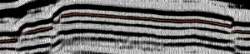
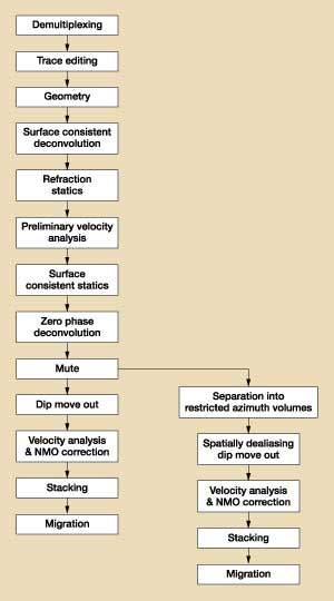
Aligned vertical faults and fractures cause azimuthal variations in seismic properties. Conventional, standard 3-D processing sequences typically stack all azimuths and thus obliterate the azimuthal variation of moveout and amplitude. Discussed here is a methodology for detecting faults and fractures in 3-D seismic data by taking advantage of the azimuthal variation of seismic signatures and coherence.

Introduction

The understanding of faulting in hydrocarbon reservoirs is a recognized challenge for: assessing a prospect and its size, the compartmentalization therein, reservoir simulation and, ultimately, maximizing hydrocarbon recovery. Similarly, appropriate fracture information is needed to: evaluate and rank a prospect, optimize well locations, decide on test intervals and evaluate the formation for optimum well development and reservoir management.¹ Routine acquisition of 3-D, high-quality seismic data, and its eventual interactive interpretation on workstations, has helped immensely in resolving faults and fractures.

Accurate imaging of features in 3-D seismic volume has permitted clarity in mapping of faults. Picking fault surfaces is time consuming. They need to be marked on inlines and crosslines and then combined into fault surfaces. However, interpretation of faults can be carried out, if their location and throws are discernible, Fig. 1. Smaller faults may have a minute reflector offset, in most cases appearing as an inconsequential disruption, Fig. 2. Similarly, minor faults are usually not directly detected, but can be detected by examining localized amplitude reduction.

Fig. 1. Faults detected in seismic sections as offsets of horizon reflectors.

Fig. 2. Smaller faults have minute reflector offsets.

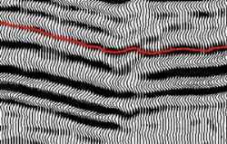
Thus, while faults with significant throws are easily marked, small or minor faults are not so evident on the seismic data volumes, even though indirect evidence (from well data or geological setting of the subsurface) does suggest the existence of faults and fractures in the area. The methodology presented here is aimed at this aspect of fault detection.

3-D seismic surveys are usually designed to record a range of azimuths. Among the various reasons for looking forward to an appreciable range of azimuths, a prominent one is the desire to image small faults and locate fracture systems.

As fault and fracture orientations vary within a prospect during acquisition of 3-D seismic data, it is intended that these features be illuminated by some of the traveling waves. Put another way, we may say that aligned vertical faults and fractures cause azimuthal variations in the seismic properties.² However, during data processing, "stacking" typically aligns all azimuths so that the azimuthal variation of moveout and amplitude get obliterated. With this in mind, it follows then that azimuth-dependent stacking would be a useful tool for seismic interpreters.

Methods Available

There are different ways of detecting small faults, e.g., using coherence, seismic attributes, etc. Coherence technology has provided interpreters a new way of visualizing faults and stratigraphic features in 3-D seismic data volumes.³ Faults produce low-coherence surfaces during the computation of 3-D coherence. They can be seen in three dimensions with the aid of visualization software, despite there having been no fault planes previously identified.

One of the most remarkable features of the Coherence Cube* is the accuracy with which faults and fractures can be visualized by simply looking at coherence time slices. Small faults may be seen on conventional, amplitude time slices, but only those running perpendicular to strike. When faults run parallel to strike, the fault lineaments get superimposed on bedding lineaments, so they become more difficult to see. The Coherence Cube reveals faults in any orientation, highlighting both parallel and perpendicular faulting equally well.

Coherence-coefficient computation is sensitive to seismic waveform changes, so it detects small faults with clarity. It is also possible to sharpen the coherence values by stretching out the range of coherence coefficients; such sharpened displays exhibit faults and fractures with greater clarity, Fig. 3. Apart from this, some visualization techniques are available on every workstation, e.g., illumination by an artificial light source. Such techniques fall in the domain of image processing. The slice under observation is treated as a topographic surface, and a change in orientation of the artificial light tends to emphasize different, low-coherence alignments.

Fig. 3. (A) Time slice from seismic volume. (B) Time slice from coherence volume depicting faults and fractures. (C) Time slice from sharpened coherence volume shows more fracture detail.

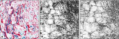
Of the many seismic attributes, amplitude envelope and frequency time / horizon slices usually indicate the faults convincingly. Fig. 4 shows seismic-coherence-amplitude envelope time and horizon slices compared with a coherence slice. Seismic attributes computed during a multitrace, semblance-based coherency computation are more robust,⁴ so they have been used in the displays. Offsets of faults cause a break in the reflections, and the seismic attribute makes them stand out clearly.

Fig. 4. (A) Time slice from coherence volume at 1,536m. (B) Time slice from coherence envelope volume at 1,536m. (C) Horizon slice from coherence envelope volume flattened on a marker horizon and 60 ms below it.

These methods work well for small faults or those with appreciable offsets of reflector horizons on seismic sections. Faults that manifest as localized amplitude changes (on closer examination) may not be detected by these methods. The following methodology has been developed for their detection.

New Methodology

The methodology presented here was applied to two different 3-D seismic volumes, a land data set from Western Canada and a West Africa OBC data volume. One conventionally processed volume did not show any plausible fault pattern that could explain the waning of initial pressure levels in and around a well drilled in the area. The other had a high density of faults. The results for both the seismic volumes are reported here.

Example 1. The conventional, standard processing sequence applied to the 3-D data volumes is shown in Fig. 5. After application of surface-consistent statics and zero-phase deconvolution to the CDP gathers, they are binned into four different azimuth volumes according to the direction between source and receiver, but within 45° of dominant fault strike. The range of azimuths fixed for each volume is 45 – 90°, 90 – 135°, 135 – 180° and 180 – 225°. Thereafter, processing was carried out independently for each of the four volumes. This included spatially dealiasing dip moveout ⁵((DMO), velocity analysis and stacking.

Fig. 5. Conventional and modified processing sequences.

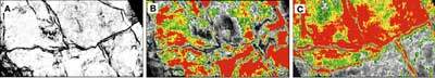
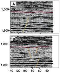
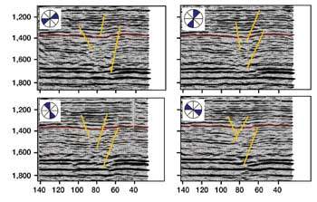
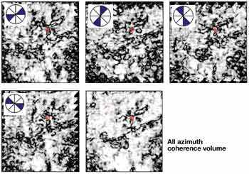
DMO should preserve the seismic amplitudes. To achieve this objective, a number of issues have to be addressed: binning of the input data to ensure that the offset classes are balanced, spatial sampling of the DMO operator, and DMO-oriented weighting of the DMO stack to compensate for effects of acquisition geometry on stack amplitudes. In the spatially dealiasing DMO algorithm used, instead of summing a DMO response to the nearest bin center, the trace is weighted and summed to the four bin centers, which are the corners of the smallest rectangle containing the response trace.⁵ The weighting is determined by distance from response trace to bin center.

Different azimuth subvolumes were analyzed through the eyes of coherence. Coherence Cubes were run on the different azimuth volumes using the modified eigen decomposition algorithm,⁶ a five-sample eigen operator and spatial radius equal to a bin length.

Fig. 6 shows inline 91 and crossline 97 from the all-azimuth seismic volume. Fig. 7 shows crossline 97 from the different azimuth-restricted volumes. As expected, there is variation in the reflection event distribution and more detail in the restricted azimuth sections, compared with conventional sections. This detail is not so pronounced on the seismic time slices. Fig. 8 shows the horizon slices (at 30 ms below the marker horizon in the zone of interest) from the corresponding coherence volumes. A system of faults in the NE – SW direction is seen on the conventional time slice but is not so distinct. Different azimuth coherence slices show better alignment not only in the NE – SW direction, but in the orthogonal direction as well. Well W1 is now seen to be located within a faulted area. This helps explain the waning of pressure initially observed in the well.

Fig. 6. (A) Inline 91 from all-azimuth seismic volume. (B) Crossline 97 from all-azimuth seismic volume.

Fig. 7. Crossline 97 from four azimuth-restricted seismic volumes. Azimuth range for each volume is indicated.

Fig. 8. Horizon slices from four azimuth-restricted coherence volumes, with azimuth ranges marked, and from all-azimuth seismic coherence volume, 30 ms below marker horizon in the zone of interest.

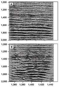
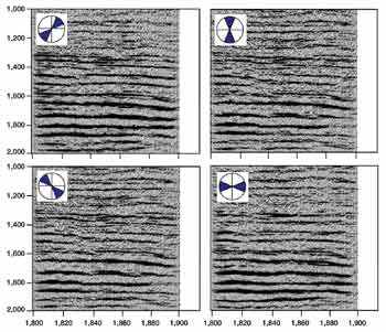
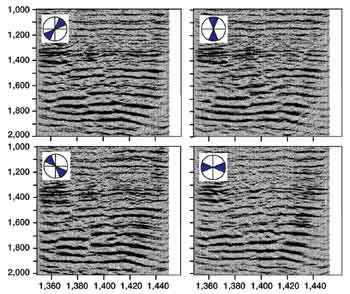
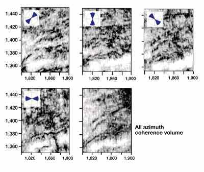
Example 2. Based on the orientation of faults in this volume, the range of azimuths fixed for each volume is 22.5 – 67.5°, 67.5 – 112.5°, 112.5 – 157.5° and 157.5 – 202.5°.

Fig. 9 shows inline 1,400 and crossline 1,830 from the all-azimuth seismic volume. Fig. 10 shows inline 1,400 from the different azimuth-restricted volumes. Similarly, Fig. 11 shows crossline 1,830 from aziumuth-restricted seismic volumes. As expected, there is variation in the reflection event distribution and more detail in the restricted-azimuth sections, compared with the conventional sections. This detail is not so pronounced on the seismic time slices. Fig. 12 shows the time slices at 1,312 ms from the corresponding coherence volumes. Some NE – SW faults are seen on the conventional time slice, but are not so distinct. Different aziumuth coherence slices show better alignment not only in the NE – SW direction, but in the orthogonal direction as well. A distinct cross fault is seen on the 157.5 – 202.5° azimuth volume.

Fig. 9. (A) Inline 1,400 from all-azimuth seismic volume. (B) Crossline 1,830 from all-azimuth seismic volume.

Fig. 10. Inline 1,400 from four azimuth-restricted volumes. Azimuth range is as indicated.

Fig. 11. Crossline 1,830 from four azimuth-restricted volumes. Azimuth range is as indicated.

Fig. 12. Time slices at 1,312 ms from four different azimuth-restricted coherence volumes, as marked, and the all-azimuth coherence volume.

An important observation is that, despite significantly lower fold of the restricted azimuth volumes, superior imaging is seen in the fracture-perpendicular direction. This result is intuitive to standard practices and suggests that both the fault-parallel and fault-perpendicular volumes need to be analyzed for accurate fault interpretation.

Conclusions

The four-azimuth method detects azimuthal anisotropy with arbitrary orientation much better than the all-azimuth stacking method. Restricted-azimuth, 3-D seismic volumes (when analyzed with coherence) offer superior imaging of fault systems in different orientations. It is a little more costly; it also requires higher processing effort and produces lower fold and S/N ratio (than conventional volumes). This is tolerable due to the high multiplicity of 3-D data, and also due to the spatially dealiasing DMO algorithm, which tends to take care of the amplitude preservation and aliasing. This methodology could be very significant for identifying zones where productivity is influenced by fractures and faults.

Literature Cited

1. Jones, G., Q. J. Fisher and R. J. Knipe, Eds., Geological Society Special Publications, No. 147, 1999.
2. Grimm, R. E. et al., "Detection and analysis of naturally fractured gas reservoirs," Geophysics, Vol. 64, No. 4., pp. 1277 – 1292.
3. Bahorich, M., and S. Farmer, "The Coherence Cube," The Leading Edge, Vol. 14, No. 10, 1995, pp. 1053 – 1058.
4. Marfurt, K. J. et al., "3-D seismic attributes using a semblance-based coherency algorithm," Geophysics, Vol. 63, No. 4, 1998, pp. 1150 – 1165.
5. Beasely, C. J., and E. Mobley, "Spatial dealiasing of 3D DMO," Expanded Abstracts, 67th Annual International Meeting SEG, 1997.
6. Marfurt, K. J. et al., "Coherency calculations in the presence of structural dip," Geophysics, Vol. 64, No. 1, 1999, pp. 104 – 111.

The authors

	Satinder Chopra specializes in Coherence Cube processing and inversion at Scott Pickford, Calgary. He obtained the M. Phil. in physics in 1978 from Himachal Pradesh University and joined Oil and Natural Gas Corp., India, in 1984. He has 15 years’ experience in the fields of seismic processing and interpretation, specializing in depth imaging, inversion and AVO analysis. He is a member of SEG, CSEG and EAGE.
	Vasudhaven Sudhakar is president of Scott Pickford, Canada, and VP of Seismic Technology for Core Lab Reservoir Management Services Division. After graduating from Madras University in 1979, he joined GSI Singapore, and he managed Halliburton Geophysical’s processing center from 1984 to 1990. He worked at the company’s R&D Department before co-founding Coherence Technology Co. He is a member of SEG and CSEG.
	Glen Larsen is a seismic processing leader at Scott Pickford, Calgary. He holds a BSc in geophysics from the University of Calgary. He specializes in 2-D/3-D land data processing. He is a member of SEG and CSEG.
	Henry Leong is seismic processing team leader at Scott Pickford, Calgary. He received the GSC from the University of Calgary in 1983. He joined Integra Geoservices, Calgary, in 1991 as a processing geophysicist, with focus on 2-D/3-D processing and software testing. He specialized in 3-D processing and has developed several techniques to integrate geological information into 3-D seismic processing.