What causes distortions on prestack reflection seismic data?

In this case study, transmission distortions are observed on prestack seismic data at two locations in the Gulf of Mexico. These distortions produce anomalous AVO signatures that result from interference patterns

Paul J. Hatchell, Shell Offshore Inc.

ransmission effects have large impacts on seismic data fidelity. For example, shallow-gas wipeout zones and fault shadows are common artifacts of seismic data. Localized distortions generate characteristic patterns on displays of reflection amplitudes (or arrival times) in the offset vs. common-midpoint (CMP) domain.

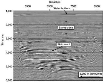
In this article, distortion zones are observed on prestack seismic data at two Gulf of Mexico locations. Their locations are determined using acquisition geometry and raytracing. No obvious reflection events, such as shallow gas zones, are observed at the predicted locations of the distortion zones. Instead, the distortion zones correlate with buried faults and unconformities.

It is postulated that the distortions are produced by velocity changes across buried faults and unconformities. The distortions are then due to an interference pattern resulting from seismic waves arriving from different sides of the faults. A simple model is developed that explains many characteristics of the distortion pattern.

Introduction

Kjartansson (see also, Claerbout) showed that prestack seismic reflection data contain significant information on transmission properties of sediments overlying reflection events.^1,2 Assuming that transmission effects are cumulative along a given seismic raypath (i.e., ignoring wavefront character), images of the transmission distortion as a function of CMP and depth were generated. Harlan recognized that these transmission distortions have a significant impact on the analysis of seismic amplitudes vs. offset (AVO) and devised a method for correcting the amplitude distortions.³

In the previous examples, the predicted locations of the distortions were only partially related to known subsurface features. Both papers relied on 2-D seismic data and presented only images along a single seismic traverse. Both Harlan and Kjartansson commented that lateral velocity variations could explain some of the observed distortion. If the velocity variations are important, then the seismic wave character must be considered, and the assumption of cumulative transmission effects along a raypath is no longer valid.

In this article, transmission distortions are observed on migrated 3-D prestack seismic data at two different locations and geological settings in the Gulf of Mexico. Depths and positions of the distortion zones are determined by analyzing reflection-event amplitudes and arrival times in the offset vs. CMP domain. In both examples, depths of the main distortion zone are not found to vary significantly with spatial position. Maps of distortion strength are generated by summing along trajectories in the offset vs. CMP domain, which are determined based on depth of the reflection event, depth of the distortion zone and acquisition geometry. The distortion zones are found to correlate with faults and unconformities.

Fagin presented an example of seismic distortions resulting from growth faults in the Wilcox trend of south Texas.⁴ His analysis showed that these distortions resulted from time sags and time pull-ups occurring from the faulting and consequent structural thinning of the high- and low-velocity layers of the Wilcox. In the two Gulf of Mexico examples, no such high- and low-velocity layers exist. Instead, the average velocity changes slowly with depth.

The distortions seen in the Gulf of Mexico examples can be explained by velocity changes across faults and unconformity surfaces that result from changes in fluid pressures and compaction at these boundaries. A simple model is developed that incorporates lateral velocity changes across a vertical boundary, and the distortions produced within the model closely match those from the observed data.

Deepwater GOM Example

The first example is from a 3-D seismic data volume acquired over the Shell / BP Mars field in 900-m (3,000-ft) waters. A 3-D AVO dataset was generated over a subset of this volume by applying common-offset dip moveout followed by common-offset time migration.

Mars basin geology comprises Miocene-age ponded turbidites (below 3,000 ms) overlain by a Pleistocene-age deepwater-canyon levee system with channel-margin slumping (1,600-2,800 ms). The slump zone is structurally and stratigraphically complex, and comprises several rotated fault blocks and channel-cut unconformities. A particularly bright reflection in the turbidite section is the pink event, which occurs just above 4,000 ms. Well control shows that this event is created by an approximately 25-m-thick oil sand. Fig. 1 shows a migrated, stacked seismic section along inline 1152.

Fig. 1. Deepwater Gulf of Mexico: migrated stacked seismic section along in-line 1152.

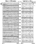
Reflection amplitudes near the pink event show unexpected amplitude fluctuations at various offset ranges. These distortions move systematically with crossline position. Several NMO-corrected, migrated CMP gathers from inline 1152 are shown in 200-ms windows centered around the pink event, Fig. 2. The crossline locations vary from 6000 to 6600, with 150-m spacing between successive panels. On the right side of the figure are plots of maximum trough amplitudes at the pink event vs. common offset for each CMP gather.

Fig. 2. NMO-corrected migrated CMP gathers (left) and snapped trough AVO (right) at several crossline locations along inline 1152. Click for enlarged view

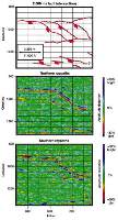
There are obvious amplitude distortions that move systematically with crossline position. In some places, the event amplitudes are anomalously strong; in others, they are anomalously weak. It is also evident that a time sag occurs on the traces where the amplitude is weak.

Another method for displaying amplitude and time distortions is to plot the peak amplitude (or time) deviation from the average amplitude (or time) in the offset vs. CMP domain. Normalizing these amplitude-deviation displays by the average amplitude also removes lateral changes in reflection strength. The distortions are clearly visible on these displays as diagonal features which move toward both increasing and decreasing crossline values as the offset distance is increased.⁵

In Fig. 2, the most prominent amplitude distortion is a bright zone paired with a dim zone. The magnitude of the amplitude distortion is about 70% and is nearly identical whether it arrives at the near or the far offsets. This distortion is likely due to focusing and defocusing of the seismic wave from laterally changing velocities.

These distortion patterns have been discussed by previous authors and are attributed to lateral changes in transmission properties of shallower sediments.^1,2,3 In this sense, the distortions are "shadows" that arise from buried anomalies in the subsurface. The slope of the distortion pattern in the offset vs. CMP domain is determined by the anomaly depth. In general, raytracing is required to evaluate the relationship between the anomaly depth and affected CMP locations.

The model trajectory which best matches the data in Fig. 2 is for an anomaly depth near 1,800 ms. Similar distortions are observed on displays generated from other inline locations; the majority of these are also consistent with anomaly depths near 1,800 ms. What is special about 1,800 ms? There are no obvious reflection events on the stack data corresponding to this location.

The predicted depth corresponds to the top of a regional slump zone in the Mars basin. Maps of the distortion strength are found to correlate with faults and unconformities in this zone. It is proposed that seismic velocity changes due to unconformity boundaries and pressure differences at the fault create the distortions. In this case, the anomalies would be useful in flagging potentially pressured fault blocks in the slumped zone. This would be a valuable tool, because unexpected pressures are often found while drilling through shallow sediments in the deepwater GOM, and some have resulted in abandonment of multimillion-dollar wells.

GOM Shelf Example

The second example is from a seismic dataset acquired in 8 m (25 ft) of water on the Gulf of Mexico Shelf. This data was acquired using ocean-bottom-cable receivers and airgun sources, which were shot parallel to the receivers with little crossline offset. A migrated 3-D AVO dataset was generated, comprising 28 offsets from 450 m (1,500 ft) to 5,900 m (19,300 ft).

In the offset vs. CMP domain, a normalized amplitude display for reflections from a sandstone horizon near 2,500 ms shows large amplitude distortions; these follow diagonal trajectories similar to those in the previous example. Model trajectories reveal the depth of the distortion to be near 2,000 ms. A growth fault is observed at the predicted location.

Anomaly maps (shadow maps) that show the location and strength of the distortions are generated by summing normalized amplitude deviations along the model’s diagonal trajectories. Two independent maps are generated, corresponding to whether the anomaly affects the raypath on the up-cable or down-cable side of the zero-offset CMP position.

Kjartansson and Harlan used similar techniques to generate distortion images in time and depth along 2-D seismic traverses. Both authors summed the results of the two raypaths to produce a single distortion image.^1,3 In the present work, contributions from the two raypaths are displayed separately for several reasons. First, they provide independent corroboration of each other. Second, errors in anomaly depths produce undesirable cancellations when the two raypath contributions are summed. Lastly, it is expected that distortions due to extended anomalies will depend on orientation of the raypaths.

Anomaly maps generated using normalized RMS amplitude deviations are displayed in Fig. 3. Maps generated from northern (up-cable) and southern (down-cable) raypaths are very similar, and each has a pronounced dim zone which is paired with a bright zone. The patterns in the anomaly maps closely match portions of the 2,000-ms, interpreted fault-plane intersections displayed at the top of Fig. 3. Close examination reveals that some of the interpreted fault-plane intersections are nearly coincident with the dim zones of the anomaly maps. Not all faults, however, are associated with an anomaly; only a few fault branches produce the anomalies.

Fig. 3. 2,000-ms fault-plane intersections (top) and anomaly maps generated using the "northern" (middle) and "southern" (bottom) raypaths. Click for enlarged view

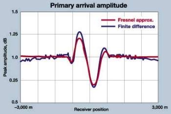
In view of the fact that the anomaly maps of Fig. 3 represent either the down-going or up-going vertically transmitted wavefield amplitudes, it is clear that the observed anomalies can affect interpretation of seismic amplitudes, especially prestack amplitudes.

Similarity between the anomaly maps and the fault patterns show that the two are related. Several questions then arise: What is the mechanism which occurs at the fault boundaries that creates the distortions? Why do the distortions come from 2,000 ms as opposed to some other depth? Why are only some faults involved and not others? A simple model is developed next, providing answers to some of these questions.

Lateral Velocity Changes

A simple model incorporating changes in seismic velocity at a boundary (such as a fault or unconformity) is developed; it predicts distortions similar to those observed in the two previous data examples.

The case where a velocity change is encountered at a vertical boundary is considered. The model comprises a constant-velocity medium, V – except for a single slow-velocity layer of thickness, T and velocity (V – DV) – which is present on only one side of the vertical boundary. Shots are located at the top of the model and receivers at the bottom.

The response at the receivers from a point source is calculated, approximately, by breaking the incident wavefield into two halfspaces, which include and exclude the slow-velocity layer. Response at the receiver location then results from interference of the two knife-edge Fresnel diffractors – one of which acquires a phase shift from the slow-velocity layer.

A comparison of primary-arrival amplitudes from synthetic seismograms – generated using the classical Fresnel approximations and a finite-difference numerical calculation – is shown in Fig. 4. The model comprises a single shot at 150-m depth and receivers at 6,000-m depth. The model velocity is a constant 1,830 m/s, except for a single slow-velocity layer at 3,000-m depth, which has a 150-m thickness and a velocity of 1,650 m/s. The slow-velocity layer is present only in the halfspace to the left side of the shot location. Receivers extend 3,000 m on either side of the vertical boundary.

Fig. 4. Arrival amplitudes with a lateral velocity change.

The amplitude distortion pattern in Fig. 4 is a bright zone paired with a dim zone, with the bright zone occurring on the slow side of the boundary. Conceptually, the velocity interface bends the incident wavefield so that energy is focused toward the slow side of the interface, which results in less energy arriving on the opposite side. In time-migrated models of reflection data, the bright zone is found on the fast side of the model.

In summary, a simple model in which the seismic velocity changes at an interface explains many of the characteristics of distortion patterns in the real data. The model predicts that energy from an incident seismic wave is focused toward the slow side of the boundary. After time migration, the bright side of the interface is the fast side of the boundary. The magnitudes of amplitude distortion and time shifts predicted by the model are in close agreement with the two data examples.

Conclusion

Amplitude and time distortions are observed on prestack seismic reflection data at two locations in the Gulf of Mexico. The distortions occur from seismic wave transmission through buried anomalies. Depths and positions of the anomalies are determined by raytracing and then compared to features in the subsurface. No obvious reflection events, such as shallow gas zones, are observed at the predicted location of the anomalies. Instead, the anomaly positions correlate with faults and unconformities.

It is suspected that the distortions are the results of seismic velocity changes across faults (or unconformities). Seismic wave propagation through a simple model, incorporating a sudden velocity change at a vertical boundary, is studied and found to reproduce the main features of the observed amplitude and time distortions.

The observed and predicted amplitude distortions are as large as 70%; they comprise paired, dim and bright zones that result from defocusing and focusing of seismic energy. These distortions complicate amplitude interpretation. Anomalous AVO signatures are produced by the distortions.

Acknowledgment

The author thanks all the people who have assisted him throughout the years with this work. Mark Rosenquist (SEPTCo) masterminded processing of the deepwater dataset, and Susan Smith (SEPTCo) kept his disks full. Mark Juedeman (SOI) contributed a number of useful suggestions in the deepwater example. Hing Tan (SOI) produced the finite-difference calculation. Robert Johnson (SOI) migrated the model calculations. Donald Zaengle (SOI) and Fred Diegel (SOI) provided geological tutoring on the Gulf of Mexico. Robert Johnson and Laura Lepre (SOI) flawlessly managed the data import and export in the shelf example. David DeMartini (SEPTCo) and Jim Robinson (SEPTCo) provided important guidance in the early days of this work.

The Shelf seismic data is courtesy of Fairfield Industries. The author thanks Shell Offshore Inc. for providing time and permission to publish this work.

This paper was first presented at the SEG 69th Annual Meeting in Houston, Oct. 31 – Nov. 5, 1999, where it won the Best Paper Presented award.

Literature Cited

1. Kjartansson, E., "Attenuation of seismic waves in rocks and applications in energy exploration," PhD thesis, Stanford University, 1979.
2. Claerbout, J. F., "Imaging the Earth’s interior," Blackwell Scientific Publications, 1985.
3. Harlan, W. S., "Tomographic correction of transmission distortions in reflected seismic amplitudes," 64th Annual Internat. Mtg., SEG, Expanded Abstracts, pp. 968 – 971, 1994.
4. Fagin, S., "The fault shadow problem: Its nature and elimination," The Leading Edge, Vol. 15, pp. 1005 – 1013, 1996.
5. Hatchell, P. J., "Fault Whispers, Transmission distortions on prestack seismic reflection data," Geophysics, Vol 65, No. 2, pp. 377 – 389, March – April 2000.

The author
	Paul J. Hatchell earned his PhD in 1989 in theoretical physics from the University of Wisconsin. He spent seven years at Shell’s Bellaire Technology Center researching and developing shear-wave logging technology, rock properties, quantitative seismic amplitude analysis and 3-D AVO applications. Following this, he transferred to Shell Offshore Inc. and spent four years pursuing oil and gas exploration in the Gulf of Mexico. Paul is currently working with Shell International E&P in the Netherlands as a member of Shell’s 4-D seismic implementation team.