Growth in conventional fields in high-cost areas: A case study

The U.S. Gulf of Mexico has produced longer than other worldwide offshore areas. Its field-growth profile may be indicative of other international offshore provinces

Emil D. Attanasi, U.S. Geological Survey, Reston, Virginia

xploration managers commonly base future drilling decisions on past experience in an area. To do this well, they should consider both discovered and undiscovered resources to characterize total future potential. Discovery-size estimates should be adjusted to account for future field growth; otherwise, the relative efficiency of recent exploration will be undervalued.

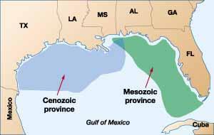
This study models and projects field growth for pre-1997 discoveries in the U.S. Federal Gulf of Mexico (GOM) Outer Continental Shelf (OCS). Projected additions to reserves for these fields from field growth through 2020 are 5.2 billion bbl of oil and 46 Tcfg. Projections include growth associated with sizable new oil discoveries in deepwater areas and initial reserve additions from new subsalt plays discovered through 1996.

This article focuses on the U.S. GOM because it has produced longer than other worldwide offshore areas. Its field-growth profile may be prototypical of other offshore provinces such as the North Sea, Scotian Shelf and deepwater Angola, as well as high-cost onshore areas.

Introduction

Government leaders want predictions of reserve discoveries and additions to project future production as accurately as possible. Near- and intermediate-term production forecasts depend on current and projected proved-reserve levels. The accepted standard for calculating and reporting proved reserves narrows the volume of hydrocarbon resources to well-defined producibility criteria.¹ For the last two decades, the main source of proved reserves additions has been from known fields, or "field growth."

Field growth is the phenomenon of increasing estimates of known recoverable hydrocarbons (past production plus current proved reserves) that occur as oil and gas fields are developed and produced. Fields are commonly defined as areas comprising single or multiple reservoirs grouped or related to the same geologic structural feature and/or stratigraphic condition. In practice, field sections may only be generally related. Field definitions may change over time due to regulatory and ownership issues and are sometimes an artifact of the historical discovery process.

U.S. fields have shown vigorous growth. The Securities and Exchange Commission originally developed the generally accepted, proved-reserve calculation procedure to standardize reported volumes of in situ oil and gas used in commercial transactions.² Resulting proved-reserve estimates and derived estimates of known field recovery (past production plus proved reserves) are conservative by design.

Early efforts to quantify field growth focused on recent discoveries – determining their fully developed size to better evaluate the effectiveness of ongoing exploration. Now that field growth is recognized as an important source of proved-reserves additions, projections of both quantity and timeliness of these additions are important for industry and government planning.

Field growth in offshore areas has not been extensively investigated.^3,4 In fact, some analysts are very skeptical about the potential significance of field growth. They argue that in high-cost areas, operators delineate and define field limits more precisely before development, so that incremental additions to ultimate field recovery will be limited.⁵

Study Area

Federal jurisdiction of the GOM OCS starts 3 mi seaward from the state shoreline. Minerals Management Service (MMS) evenly divides the 249,000-sq-mi area into two petroleum provinces, Fig. 1. Discoveries in the Cenozoic area account for virtually all past OCS production, while the Mesozoic accounts for about 5% of gas reserves.³ Through 1997, the Federal GOM OCS has produced 10.8 billion bbl of oil and 133.8 Tcfg.

Fig. 1. Petroleum provinces of U.S. Federal GOM OCS according to MMS.

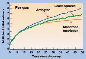
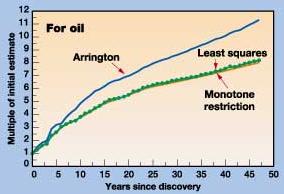
Data

There are very few case histories for which field-size estimates – from year discovered to year abandoned – are available. Available data are generally short series of estimates of ultimate-field recovery grouped by discovery year.

To provide a basis for tracking field growth, the Energy Information Administration (EIA) developed the Oil and Gas Integrated Field File (OGIFF) from proprietary industry responses to form EIA-23 (Annual Survey of Domestic Oil and Gas Reserves). This file comprises field records that include annual estimates of known crude oil and wet-gas recovery since 1977.

For calculation purposes, fields that straddle state/federal boundaries were classified based on where the majority of their hydrocarbon resources lay. Fields were classified as non-associated gas if the estimated ratio of gas/oil recovery was at least 20 Mcf/bbl; otherwise, a field was considered an oil field. This ratio ensured that fields classified as non-associated gas were developed as gas.

Discoveries And Past Field Growth

In more than 1,000 fields in federal waters, about 15.5 billion bbl of oil and 178.9 Tcfg had been discovered through 1996. Nearly 32% of this gas was in oil fields. From 1977 to 1996, estimates of known oil and gas recovery in pre-1978 discoveries grew by 4.6 billion bbl oil and 50 Tcfg. That is, during the 20-yr period, known recovery in pre-1978 discoveries grew 58% for oil and 53% for gas.

Modeling Field Growth

If fields are grouped by discovery year, the sum of the estimates of known recovery for each group usually increases as time passes. The increases were roughly systematic and suggested a statistical modeling approach. If i is the number of years after discovery, the annual growth factor for year i, or equivalently for fields i years old, is the ratio of the estimated field size made in year i + 1 to the estimated field size made in year i.

A cumulative growth factor is the ratio of the size of the field, n years after discovery, to the initial estimate of field size.

For subsequent years, the cumulative growth function (represented by a set of yearly cumulative growth factors) can be used to project field-size estimates.

Individual growth factor: Calibration approach. Arrington published the first study to apply growth factors to adjust recent discovery sizes.⁶ He computed the annual growth factor for the n+1 year after discovery as the sum of estimates of known recovery of fields at age n+1, divided by the sum of the estimates of known recovery of the same fields at age n.

Cumulative growth factors were computed by multiplying annual growth factors for successive years. Marsh and Root applied the Arrington technique to project field growth at the national level.^7,8

Joint growth factor: Calibration approach. All cumulative growth coefficients can be estimated simultaneously by choosing a set of coefficients that minimizes the sum of squared errors (residuals).

The cumulative growth function that results from minimizing the sum of squared deviations for the entire set of coefficients is called the least squares growth function. By further imposing the condition that the percentage growth of older fields will not exceed the percentage growth of younger fields, then the growth function has a monotonic shape, i.e., smoothly increasing, non-oscillating.

Growth functions. Cumulative growth functions were calibrated using yearly known recovery estimates (1977 through 1996) of conventional, federal Gulf OCS fields, grouped by discovery year from 1947 to 1996. Figs. 2 and 3 show cumulative growth functions for oil and gas, respectively. Each figure presents the cumulative growth function calculated with three methods: 1) Arrington, 2) least squares, and 3) least squares with monotonic condition.

Fig. 2. Cumulative growth functions for oil in oil fields. Based on OGIFF file, 1998.

Fig. 3. Cumulative growth functions for gas in gas fields. Based on OGIFF file, 1998.

Criteria for choosing the set of cumulative growth functions for projection of reserve additions were: 1) how well does the model fit the data; and 2) does the resulting function conform to intuition?

By definition, the least squares set of coefficients was picked to minimize the sum of squared residuals. Table 1 shows the sum of squared residuals (calculated as the square of the quantity of the predicted-minus-actual estimate) over all possible combinations of field age and year of estimate for each model. The sum of squared residuals represents the magnitude of variation left unexplained by a particular model. The imposed monotone condition only slightly increases the sum of squared residuals, but the sum of these squared errors was significantly larger with the Arrington model.

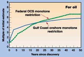
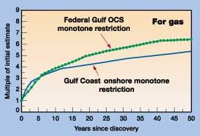
As a way to illustrate this, suppose that fields did not grow. In that case, all growth factors would equal one. Further, suppose that the sum of squared residuals (for a particular growth model) divided by the sum of squared residuals (assuming "no growth") was interpreted as the percent of variation not explained by the model relative to the "no growth" hypothesis. The difference between this ratio and 100% will be interpreted as the fraction of variation explained by a specific growth model. These values are shown in the Table 1 column designated "explanatory power."

Generally, gas cumulative-growth functions had higher explanatory power than oil growth functions. Least squares had the highest explanatory power, followed by the monotone constraint on least squares, while the Arrington model had the weakest power.

The second criterion for model choice was conformance to intuition. At one or more ages (years after discovery), both the oil and gas least squares models implied that fields actually shrank in size. Both the monotone-restriction model and the Arrington model were well behaved and did not have this problem. Hence, the monotone-restriction model was used for projecting reserve additions from field growth.

Are development profiles captured by the growth functions for onshore and offshore fields different? Figs. 4 and 5 show the cumulative field-growth functions with the monotone restriction for oil and gas in the federal Gulf OCS. Similar functions were computed with data from the Gulf Coast Region onshore and state waters. In this comparison, only conventional fields were used in the cumulative growth-function calibration.¹⁰

Fig. 4. Cumulative growth functions for oil in oil fields for the Federal GOM OCS, Gulf Coast onshore and state offshore waters.10

Fig. 5. Cumulative growth functions for gas in gas fields for the Federal GOM OCS, Gulf Coast onshore and state offshore waters.10

Onshore cumulative-growth functions initially increase more rapidly than functions for federal offshore fields. Offshore field delineation continues in the years following discovery, but production is commonly delayed until production-platform installation. Onshore, field development and production occur quickly after discovery. Thus, the curves confirm what is intuitively known to be true about onshore and offshore field-production practice.

Field Growth Projections

Cumulative-growth functions with the monotone restriction (Figs. 2 and 3) were applied to 1996 estimates of field size (known recovery) to project future reserve additions from pre-1997 discoveries through 2040. Co-product forecasts (associated gas, gas liquids) are derived from projections of primary products and assumptions of constant gas-to-liquids ratios in oil fields and liquids-to-gas ratios in gas fields. These ratios are based on 1996-estimated known recovery for discovered fields.

Implicit in applying the calibrated cumulative-growth function is the assumption that the technological improvement rate and economic conditions occurring during the observation period will prevail in the future. Though some assumptions may not prove true, nonetheless, the projection is an initial baseline forecast.

Through 2020, 5.2 billion bbl of oil and 46 Tcfg are projected to add to pre-1997 discoveries; additions by 2040 are estimated at 6.4 billion bbl of oil and 54 Tcfg. These numbers are not directly comparable to recent MMS estimates of 2.2 billion bbl of oil and 33 Tcfg by 2020, because MMS used growth functions computed on a boe basis for a data series ending in 1994.³ Projections presented here include growth associated with sizable oil discoveries made before 1997 in deepwater areas and initial reserve additions from new subsalt plays.¹¹ Table 2 is an annual forecast to 2040 (only every fifth year is shown), while Table 3 presents the cumulative growth factors for every fifth year.

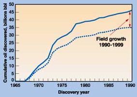
Implications

The growth-function extrapolations were limited by field-discovery age used in the analysis. Some Gulf OCS fields discovered before 1997 will undoubtedly continue to grow beyond the 40-plus years of this projection. This will occur because of improved recovery in identified pools, and because new pools will likely be added to these fields.

Ideally, to capture total cost of field growth, predictions should be burdened by field-development costs. Such an analysis might have to be at the pool or reservoir level to credibly capture economic drivers of field growth such as enhanced recovery, well recompletions and stimulation. In addition, for high-cost areas, there is an important link between field growth and infrastructure maturity. Availability of production platforms and pipeline systems with unused capacity has made possible profitable development of hydrocarbon accumulations of marginal size.

Field growth will make a substantial contribution to future reserve additions in this high-cost area. Recall that growth in known recovery is closely connected to reserve definition and reporting of initial field sizes. Reserve definitions used internationally are not as tight as the U.S. definition of proved reserves; so, one should be careful about application of the functions in situations where broader field-reserve definitions – that perhaps include substantial uneconomic resources – are included in the initial field-size estimate.

Nonetheless, there is evidence of field growth internationally. Fig. 6 shows the oil-discovery profile of fields discovered in the North Sea Graben through 1990; these fields’ sizes were estimated in 1990 and 1999. Field growth is represented as the vertical displacement across curves. During the 10-yr period, the 1996 estimates went to 46 from 35 billion bbl of oil, an increase of about 31%.

Fig. 6. Cumulative oil discovered in North Sea Graben fields through 1990. Estimates are as of 1990 and 1999 (data from Petroconsultants).

Literature Cited

1. "Definitions for oil and gas reserves," Journal of Petroleum Technology, pp. 557 – 578, May 1987.
2. "Financial accounting and reporting of oil and gas producing activities, securities and exchange commission reserves definitions, regulation S-X rule 40-10," Bowne & Co. Inc., New York, March 1981.
3. Lore, G. L., J. P. Brooks, D. W. Cooke, R. J. Klazynski, D. L. Olson and K. M. Ross, "Summary of the 1995 assessment of conventionally recoverable hydrocarbon resources of the Gulf of Mexico and Atlantic outer continental shelf: as of January 1, 1995," OCS Report, MMS 96 – 0047, 1996.
4. Drew, L. J. and G. L. Lore, "Field growth in the Gulf of Mexico – A progress report," U.S. Geological Survey Circular 1074, pp. 22 – 23, 1992.
5. Ivanhoe, L. F., "Future world oil supplies: There is a finite limit," World Oil, October 1995.
6. Arrington, J. R., "Size of crude reserves is key to evaluating exploration programs," Oil and Gas Journal, Vol. 58, No. 9, 1960.
7. Marsh, R. G., "How much oil are we really finding?" Oil and Gas Journal, Vol. 69, No. 14, 1971.
8. Root, D. H., "Estimation of inferred plus indicated reserves for the United States," in Dolton, G. L. et al., "Estimates of undiscovered recoverable conventional resources of oil and gas in the United States," U.S. Geological Survey Circular 860, pp. 83 – 87, 1981.
9. Attanasi, E. D. and D. H. Root, "The enigma oil and gas field growth," Bulletin of the American Association of Petroleum Geologists, Vol. 78, No. 3, 1994.
10. Root, D. H., E. D. Attanasi, R. F. Mast and D. L. Gautier, "Estimates of inferred reserves for the 1995 USGS National Oil and Gas Resource Assessment," U.S. Geological Survey Open-File Report 95 – 75 – L, 1996.
11. Montgomery, S. L. and D. Moore, "Subsalt play, Gulf of Mexico: A review," Bulletin of the American Association of Petroleum Geologists, Vol. 81. No. 6, 1997.

The author

Emil D. Attanasi has been an economist with the U.S. Geological Survey since 1972. His work focuses on development and application of resource assessment methods and integration of economics into USGS oil and gas assessments. He earned a BA degree in mathematics from Evangel College and a PhD in economics from the University of Missouri.